Formation Flight Computational Fluid Dynamics

     This is a post about computational fluid dynamics analysis of formation flight.

     The results from an analysis of three unmanned combat aerial vehicles (UCAVs) flying in a V-type formation are presented. The chosen UCAV configuration, shown in Figs. 1-2 and available for download here, is named SACCON (Stability And Control Configuration) UCAV. This configuration is used because of the availability of the geometric and aerodynamic data, used in the validation and verification of the numerical analysis. The SACCON UCAV is designed by NATO's (North Atlantic Treaty Organization) RTO (Research and Technology Group) under Applied Vehicle Task Group (AVT-161) to assess the performance of military aircrafts.

Fig. 1, SACCON UCAV

Fig. 2, Technical drawing for the SACCON UCAV

     The simulation is performed using commercially available computational fluid dynamics code.  The details about the solver and the discretization schemes are presented next. The simulation is performed using SIMPLE-R solver for pressure-velocity coupling. The diffusive terms of the Navier-Stokes equations are discretized using central differentiating scheme while the convective terms are discretized using the upwind scheme of second order. The κ-ε turbulence model with damping functions is implemented to model turbulence. The simulation predicts three-dimensional steady–state flow over UCAVs.

     The Reynolds and Mach number of flow are set at 1e6 and 0.15, respectively. The two trailing UCAVs are placed 3 wingspans behind the leading UCAV. The trailing UCAVs are a wingspan apart. The V-type configuration is chosen because it is the most common observation in birds (author's observation). The V-type formation is shown in Fig. 3. All three UCAVs are at 5° angle-of-attack.

Fig. 3, The V-type formation (top view)

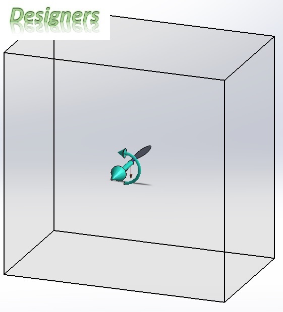
     The boundaries of the computational domain are located at a distance equivalent to 10 times the distance between the nose of the leading UCAV and the tail of the trailing UCAV. The mesh is made of 821,315 cells. Mesh controls are used to refine the mesh in the areas of interest i.e. on the surfaces of the UCAVs and in the wake of all three UCAVs. A cartesian mesh with immersed boundary method is used for the present study. The computational domain with mesh is shown in Fig. 4 while a closeup of the mesh is shown in Fig. 5.

Fig. 4, The computational domain and mesh

Fig. 5, Closeup of mesh, notice the refined wakes of the UCAVs

     For validation and verification, the lift and drag forces from the present study are compared with studies [1-2]. The results are in close agreement with [1,2] As a result of flying in a formation, an improvement in the lift-to-drag ratio of 10.05% is noted. The lift-to-drag ratio of the trailing UCAVs is at 11.825 in comparison with a lift-to-drag ratio of a single UCAV, i.e. 10.745. The lift coefficient is increased by 7.43% while the drag coefficient decreased by 2.174%. The reason(s) to why the efficiency increases will be looked upon later, if ever the author has the time and will power ☺.

     The results from post processing of the simulations are presented in Figs. 6-7. The pressure iso-surfaces colored by velocity magnitude are shown in Fig. 6. While the velocity iso-surfaces colored by pressure magnitude are shown in Fig. 7.

Fig. 6, Flight direction towards the reader

Fig. 7, Flight direction away from the reader

     Thank you very much for reading. If you would like to collaborate on research projects, please reach out.

[1] https://doi.org/10.2514/1.C031386

[2] https://doi.org/10.1155/2017/4217217

Hypersonic Flow over a Two Dimensional Heated Cylinder

     This post is about the simulation of hypersonic flow over a heated circular cylinder, in two dimensions.

     Equation 1 is used as a relationship between Mach and the Reynold number.

M= Re*μ*√(R*T) ÷ d*P*√γ     (1)

     w.r.t. equation 1, the parameters represent the following quantities.

     M     Freestream Mach number at 17.6
     Re    Reynolds number at 376,000
     μ     Dynamic viscosity at 1.329045e^-5 Ns.m^-2
     R     Specific gas constant at 286.9 J.(kg.K)^-1
     T     Freestream temperature 200 K
     d     Cylinder diameter at 5.6730225e^-4 m
     P     Freestream pressure at 101325 Pa
     γ     Specific heat ratio at 1.4
     Tw  Wall temperature of cylinder at 500 K
     Pr    Prandtl number at 0.736

     The boundary conditions were taken from [1]. A comparison with [1] is shown in Fig. 1. Inside Fig. 1, the red dotted line with circles represents the data from [1]. The black solid line represents the data from the present simulation. Within Fig. 1, 0° represents the stagnation point. The velocity, pressure, Mach number and temperature contours are shown in Fig. 2.

Fig. 1 A comparison with previous research [1].

Fig. 2, Top Row, L-R: Velocity and pressure contours. Bottom Row, L-R: Mach number and temperature contours.

The computational mesh and the computational domain with boundary conditions visible are shown in Fig. 3-4, respectively. The computational domain had a size of 20D x 20D. The mesh had 836,580 total cells and 944 cells were located at the solid fluid boundary. Several local mesh controls were employed to capture the shockwave properly.

Fig. 3, The computational mesh.

Fig. 4, The computational domain.

     The solution method is Finite Volume method. SIMPLE-R is the solver employed. Implicit central difference scheme for diffusion terms, second-order Upwind scheme for convective terms and first-order implicit for temporal terms are used. The mesh created uses the Cartesian mesh with Immersed Boundary method.

     Reference:

     [1] https://arc.aiaa.org/doi/10.2514/6.2004-2371 

     Thank you for reading. If you would like to collaborate on research projects, please reach out. I am looking for a PhD position, any guidance would be appreciated.

Computational Fluid Dynamics Analysis of a Drone

     This post is about the computational fluid dynamics analysis of a small drone. The drone features a blended body-wing design with various cross sections at different span-wise locations. The drone has a wing-span and length of 6 ft. and 4.92 ft., respectively. The root (center) portion of the drone is relatively thicker and symmetrical in cross section for increased mechanical strength while the the mid-section and wing tips are thinner and utilize more cambered aero-foils. This is purely a concept design and as of now, no physical model of this drone exists.

     The numerical simulations for the present study were carried out using SolidWorks Flow Simulation Premium© code. The code employs κ-ε model with Two-Scales Wall Functions approach as the turbulence model. The numerical algorithm implemented is the SIMPLE-R, modified. The second-order upwind discretization scheme is used to approximate the convective fluxes while the diffusive terms are approximated using the central differencing scheme. The time derivatives are approximated with an implicit first order Euler scheme. The SolidWorks Flow Simulation© solves the Navier-Stokes equations, equations 1-3, which are formulations of mass, momentum and energy conservation laws for fluid flows. Turbulent flows are predicted using the Favre-averaged Navier-Stokes equations.

     The mesh independence test was carried out starting with 348,679 fluid cells. The mesh density was then increased up to 2,360,514 cells. The results of mesh independence study are mentioned below.

                          Mesh Name             Cells            Lift [N]         Drag [N]      Lift/Drag

                          M1                          348,679       382.41 -48.14      7.95

                          M2                          1,032,665    466.08      -48.73      9.57

                          M3                          1,559,516    473.48 -47.89      9.89

                          M4                          1,990,010    486.38 -48.08      10.12

                          M5                          2,360,514    491.07 -48.32      10.16

     It can be seen that as the mesh density increased, the difference in the critical parameters between two successive meshes also reduced. The mesh independence test was stopped as the difference between all of the critical parameters was less than one percent for the meshes M4 and M5.

     The pressure and velocity plots at various span-wise locations are shown in Fig. 1-2. It can be clearly seen that there is a negligible change in the velocity and pressure distributions around the drone between meshes M4 and M5. It can also be seen that as the mesh becomes finer, the resolution of both the pressure and velocity plots also increases.

Fig. 1, Velocity contours of various meshes.

Fig. 2, Pressure contours of various meshes.

     Aero-acoustics around the drone were also examined, as shown Fig. 3.

Fig. 3, Sound level contours of various meshes.

     A zoomed in view of the computational mesh is shown in Fig. 4. The refined mesh at the drone walls as a result of the mesh controls employed is clearly visible. The hump near the root of the drone is also visible, it was added in order to prevent the span-wise flow.

Fig. 4, Mesh level M4.

     The boundary conditions and the computational domain are shown in Fig. 5. The large red arrows represents inlet velocity boundary condition and the large blue arrows represents the atmospheric pressure outlet boundary condition. The red squares represents real wall boundary condition (slip) applied to the computational domain walls so that the boundary layer from the walls does not effect the flow around the drone.

An animation of an aileron roll can be seen here.

Thank you for reading. If you would like to collaborate on research projects, please reach out.

Vertical Axis Wind Turbine Computational Fluid Dynamics Analysis

     This post is be about the validation and verification of the computational fluid dynamics analysis of a three blade vertical axis wind turbine. The turbine had a diameter of 2 m with each blade being 1 m tall. The blades had an NACA-0018 airfoil cross section.

     The computational fluid dynamics analysis employed the κ-ε turbulence model with damping functions as the turbulence model, SIMPLE-R as the numerical algorithm. The spatial discretization schemes for the convective fluxes and diffusive terms used are the second order upwind and central approximations, respectively. An implicit first-order Euler scheme is employed to approximate the time derivatives.

     The Cartesian computational mesh with immersed boundary method had a total of 769,357 cells. Among those 769,357 cells, 166,188 cells were around the turbine blades. Mesh controls were employed to refine the mesh near the turbine blades. A time step of 3e^-3 was employed. The computational domain inlet was 1.5 D away from the turbine and the outlet was 3D away. The computational domain walls on the sides were 1D x 1.5D, where D represents the turbine diameter. The mesh and the computational domain are shown in Fig. 1. The vertical teal arrow represents the force of gravity, the curved teal arrow represents the direction of turbine rotation. The dark blue arrow represents the direction of free stream velocity.

Fig. 1, Mesh and computational domain.

     The simulations ran at a tip-speed ratio of 1.87 at a wind speed of 4.03 m.s^-1. The velocity distribution around the turbine after 4 revolutions is shown in Fig. 2. Validation of the numerical analysis was carried out using [1]. The results of power produced by the turbine were with in 4% of the experimental results [1]. An animation of the numerical analysis is also shown.

Fig. 1, Flow field around the turbine.

     Thank you for reading. If you would like to contribute to the research, both financially and scientifically, please feel free to reach out.





[1] Yi-Xin Peng, You-Lin Xu, Sheng Zhan and Kei-Man Shum, High-solidity straight-bladed vertical axis wind turbine: Aerodynamic force measurements, Journal of Wind Engineering and Industrial Aerodynamics, January 2019.

Improvement of the Volume Flow Rate Through a Blower Fan

     In this post, an improvement in the volume flow rate through the blower fan assembly made are presented. The only thing changed in the blower fan was the cross section of the fan blades. In the previous version, the blade cross section resembled a flat plate with fillets at the leading edge. The trailing edge in the previous design was blunt. In the modified design, there aero-foils were selected, namely NACA 9410, NACA 9420 and the NACA 9430. All the other parameters were kept the same to the previous case. The CAD models of the modified fan blades are shown in Fig. 1.

Fig. 1, Fan blade geometries.

     The velocity contours are shown in Fig. 2 while the pressure contours are shown in Fig. 3, super imposed with velocity vectors and the computational mesh. The volume flow rate was the most for the fan with blades having cross-section of NACA 9410 aero-foil, followed by the fan with blades having cross-section of NACA 9420 and the NACA 9430 cross sections, respectively.

Fig. 2, Pressure contours. Row 1, L-R; fan with the NACA 9430 and NACA 9420 cross sections. Row 2, fan with NACA 9410 cross sections.

Fig. 3, Velocity contours. Row 1, L-R; fan with the NACA 9430 and NACA 9420 cross sections. Row 2, fan with NACA 9410 cross sections.

     Thank you for reading. If you would like to collaborate, both scientifically and financially, on research projects, please reach out.

Computational Fluid Dynamics Analysis of a Blower/Centrifugal Fan: Update 01

     In this post the results from a CFD analysis of a blower fan are presented. The fan had a diameter of 66 mm and a height of 12.57 mm. The fan's rotational velocity was at 10,000 rpm. The CAD model is shown in Fig. 1.

Fig. 1, CAD Assembly of the Blower Fan.

     The simulations were completed in SolidWorks Flow Simulation Premium code. The code employs immersed boundary method to create a Cartesian mesh. The sliding mesh feature was employed to simulate the rotation of the fan at atmospheric conditions. The code employs κ-ε model with Two-Scales Wall Functions approach as the turbulence model. The numerical algorithm implemented is the SIMPLE-R, modified. The second-order upwind discretization scheme is used to approximate the convective fluxes while the diffusive terms are approximated using the central differencing scheme. The time derivatives are approximated with an implicit first-order Euler scheme.

     The numerical model for the fan had 816,994 cells of which 209,421 cells were at the solid-fluid interface. Two mesh controls were employed to refine the mesh near the blades of the fan and at the boundary of the stationery and the rotating domains. The results were indeed, mesh independent. Due to the fact that this was an internal flow problem, domain independence test was not applicable. The mesh and the computational domain is shown in Fig. 2. The curved teal arrow represents the direction of rotation of the fan. The blue arrows represent the pressure boundary conditions at the inlet and at the outlet of the fan assembly. The straight teal arrow represents the force of gravity (the arrow is inverted).

Fig. 2, The mesh and the computational domain.

     The pressure and velocity plots are shown in Fig. 3-4.

Fig. 3, Pressure contours.

Fig. 4, Velocity contour

     Thank you very much for reading. If you would like to collaborate on research projects or want a tutorial for the setup of the numerical simulations such as this one, please reach out.

Update 01

     CAD files are available here.

Computational Fluid Dynamics Analysis of a Symmetrical Wing, Update 01

     This post is about the computational fluid dynamics analysis of a wing. The wing analyzed employed the NACA 0021 section throughout. The wing had a span of 4 m and a chord length of 1 m. The Reynolds number was kept at 3,000,000. The software employed was SolidWorks Flow Simulation Premium.

     The mesh had a total of 385,064 cells of which 84,826 cells were in contact with the wing surface, as shown in Fig. 1. The results are, indeed, mesh independent. Mesh controls were employed to refine the mesh near the wing surface. The computational domain employed was of cylindrical shape.

 

Fig. 1, The computational mesh around the wing.

 

     The velocity variation at various angles of attack around the wing cross-section is shown in Fig. 3 while the pressure variation on the wing surface is shown in Fig. 4. The results were validated against experiments conducted by [1].

 

Fig. 2, Velocity variation around the wing at 0-25 degree AOA, 5 degree increments.

 

Fig. 3, Pressure variation at the wing surface at 0-25 degree AOA, 5 degree increments.

     The purpose of this blog is maintain my online portfolio. I did this analysis because I realized I haven't written anything of this nature before. All of my previous simulations and/or blog entries were from the propulsion, renewable energy and turbo-machinery areas.
 

     Update 01

     CAD files are available here.

 

    
     Thank you for reading. If you would like to collaborate on research projects, please feel free to contact.

     [1] Fernando A. Rocha, Adson A. de Paula, Marcos d. Sousa, André V. Cavalieri, and Vitor G. Kleine, "Lift enhancement by wavy leading edges at Reynolds numbers between 700,000 and 3,000,000," Proceedings of the 2018 Applied Aerodynamics Conference, AIAA AVIATION Forum, Atlanta, GA, 2018.

     https://doi.org/10.2514/6.2018-3816

Computational Fluid Dynamics (CFD) Analysis of a Horizontal Axis Tidal Turbine (Update 01)

     In this post, the results of numerical simulations carried out on a three-blade horizontal-axis tidal turbine blades are made available. These simulations are a part of larger project relating to a horizontal-axis tidal turbine.

 

     The turbine under investigation had a diameter of 4 m. The aero-foils employed include the NACA 4424 (chord length 0.25 m), NACA 4420 (chord length 0.2312 m), NACA 4418 (chord length 0.2126 m), NACA 4417 (chord length 0.1938 m), NACA 4416 (chord length 0.175 m), NACA 4415 (chord length 0.1562 m), NACA 4414 (chord length 0.1376 m), NACA 4413 (chord length 0.1188 m) and the NACA 4412 (chord length 0.1 m) at a distance of 0.4 m, 0.6 m, 0.8 m, 1 m, 1.2 m, 1.4 m, 1.6 m, 1.8 m, 2 m from the blade root, respectively [1].

 

     The numerical simulations were carried out on SolidWorks Flow Simulation Premium software. The software employs κ-ε turbulence model with damping functions, SIMPLE-R (modified) as the numerical algorithm and second order upwind and central approximations as the spatial discretization schemes for the convective fluxes and diffusive terms. The time derivatives are approximated with an implicit first-order Euler scheme. To predict turbulent flows, the Favre-averaged Navier-Stokes equations are used. The software employs a Cartesian mesh which is created using the immersed boundary method.

 

     The simulations were carried out using the Local rotating region(s) (Sliding) technique. The mesh had a total of 589,763 cells. 132,045 cells were at the turbine blade-rotating region boundary. While the process of mesh generation, a mesh control was employed to refine the mesh near the turbine blades and at the boundary of the rotating region and the stationery computational domain. To refine the mesh for the mesh independent test, the curvature level was increased i.e. the mesh in the areas of interest was refined by a factor of 8. As a result, the refined mesh had a total of 916,577 cells. A total of 221,978 were present around the turbine blade. The computational mesh around the turbine blade is shown in Fig. 1. The refined mesh in the areas of high gradients is also clearly visible. The computational domain had dimensions of 2D x 2D x 2.4D, where D is the diameter of the turbine. The dimensions for the computational domain resemble to those in [2].

     Fig. 2 shows computational domain around the turbine blades. In Fig. 2, the curved teal arrow represents the direction of rotation of the turbine. The green arrows represent the respective co-ordinate directions. The brown arrow represents the direction of the force of gravity. The blue arrow represents the direction of the fluid velocity. The circular disc represents the rotating region.

 

Fig. 1, The computational mesh.

    

Fig. 2, The computational domain and the orientation of the boundary conditions.

 

     The simulations were carried out for a total of 5 tip-speed ratios for the turbine ranging from 2 to 10. The fluid; water, velocity was set at 2 m/s. The results are indeed, mesh independent. The mesh independence test was conducted on the design point of the turbine i.e. at the TSR of 6. The plot between the turbine tip-speed ratio; TSR, and the co-efficient of power is shown in Fig. 3. It can be clearly seen from Fig. 3 that the results are in close agreement with the results from [1, 3]. The CFD results from both studies are lower then the BEM, Blade-Element Momentum, results because the three-dimensional effects are not considered while implementing the BEM method.

 

Fig. 3, Turbine efficiency plot.

 

     Fig. 4 shows velocity streamlines colored by velocity magnitude, both of these features are drawn relative to the rotating reference frame, around the turbine blade cross-section at various tip-speed ratios. It can be seen from Fig. 4 that the turbine stalls at TSR of 2 due to a large positive angle of attack. It can also be seen that as the TSR increases, the angle of attack on the blade decreases, it is because of this reason that the power output from the turbine increases.

 

 

Fig. 4, Row 1, L-R; TSR of 2 and 4. Row 2, L-R; TSR of 6 and 8. Row 3, TSR of 10.

 

     Thank you for reading. If you would like to collaborate with research projects, please reach out.

     [1] Binoe E. Abuan, and Robert J. Howell, "The Influence of Unsteady Flow to the Performance of a Horizontal Axis Tidal Turbine," Proceedings of the World Congress on Engineering. London, 2018.

     [2] Ibrahim, I. H., and T. H. New, "A numerical study on the effects of leading-edge modifications upon propeller flow characteristics," Proceedings of Ninth International Symposium on Turbulence and Shear Flow Phenomena. Melbourne, 2015.
     [3] Bahaj, A., Batten, W., & McCann, J. (2007). Experimental verifications of numerical predictions for the hydrodynamic performance of horizontal axis marine current turbines. Renewable Energy, 2479-2490.

Update 01:

     CFD post processing added. One more TSR simulated.

Steady-State VS Transient Propeller Numerical Simulation Comparison

     This post is about the comparison between steady-state and transient computational fluid dynamics analysis of two different propellers. The propellers under investigation are 11x7 and 11x4.7 propellers. The first number in the propeller nomenclature is the propeller diameter and the second number represents the propeller pitch, both parameters are in inch. The transient analysis was carried out using the sliding mesh technique while the steady-state results were obtained by the local rotating region-averaging method. For details about 11x7 propeller click here, for the details about 11x4.7 propeller, click here.

 

     As expected, the propeller efficiencies of transient and steady-state analysis are within 0.9% of each other, as shown in Fig. 1-2. Therefore, it is advised to simulate propellers and horizontal axis wind turbines using the steady-state technique as long as no time-dependent boundary conditions are employed.

 

Fig. 1, Propeller efficiency plot.

  

 Fig. 2, Propeller efficiency plot.

 

     It can be seen from Fig. 3-4 that time taken by the steady-state simulation to converge is on average 42.37% less that the transient analysis.  The steady-state analysis takes considerably less time to give a solution then a transient analysis.

 

Fig. 3, Solution time.

 

Fig. 4, Solution time.

 

Thank you for reading. If you would like to collaborate on research projects, please reach out.

11x7 Aeronautic Propeller Characteristics (Using CFD) (Verified and Validated) (Update 02)

     This post presents the results from an aeronautic propeller CFD analysis.

    
     An 11x7 propeller was modelled using SolidWorks CAD package using the geometry from [1]. The simulations were run at two different rotational velocities and each rotational velocity was simulated at three advance ratios. The mesh for the 3,000 RPM rotational velocity had 213,205 total cells among which 24,048 cells were at the solid fluid boundary. While, the mesh for the 5,000 RPM rotational velocity had 369,963 total cells among which 68,594 cells were at the solid fluid boundary. A mesh control was employed to refine the mesh near the propeller geometry and at the boundary of the rotating region and the stationery domain for all of the cases simulated. This was done to ensure accuracy of the results was within an acceptable range. The results of the numerical simulations are plotted along with the experimental results [1] in Fig. 1.

Fig. 1 J= Advance Ratio, η_prop = propeller efficiency

     It can be seen from Fig. 1 that the trends for the propeller efficiency are in agreement with the experimental results. To increase the mesh density for the mesh independence test, the number of cells in  each of the respective co-ordinate directions was increased by a factor of 1.1. The mesh is shown in the Fig. 2.

Fig. 2 The computational mesh around the propeller.

     The computational domain size was at 2D x 2D x 2.4D, D being the propeller diameter, as shown in Fig. 3. In Fig. 3, the curved teal arrow represents the direction of rotation of the sliding mesh. The blue arrow represents the direction of free stream velocity while the brown arrow represents the force of gravity.

 Fig. 3 The computational domain.

Fig. 4 The pressure distribution and the velocity vectors around the propeller.

     The CAD model files and the simulation setup files for the numerical analysis are available here.

     Thank you for reading. If you'd like to collaborate on research projects, please reach out.

[1] Brandt, J. B., & Selig, M. S., “Propeller Performance Data at Low Reynolds Numbers,” 49th AIAA Aerospace Sciences Meeting, AIAA Paper 2011-1255, Orlando, FL, 2011.

doi.org/10.2514/6.2011-1255

 

Update 01

     Results from the mesh independent study are now available.

Update 02

     CAD model files are now uploaded. The CFD simulation setup files are also included.

11x4.7 Aeronautic Propeller Characteristics (Using CFD) (Verified and Validated) (Update 02)

     This post presents the results from an aeronautic propeller CFD analysis.

     An 11x4.7 propeller was modelled using SolidWorks CAD package using the geometry from [1]. The simulations were run at two different rotational velocities and each rotational velocity was simulated at three advance ratios. The mesh for the 3,000 RPM rotational velocity had 206,184 total cells among which 22,103 cells were at the solid fluid boundary. While, the mesh for the 6,000 RPM rotational velocity had 357,300 total cells among which 64,012 cells were at the solid fluid boundary. A mesh control was employed to refine the mesh near the propeller geometry and at the boundary of the rotating region and the stationery domain for all of the cases simulated. This was done to ensure accuracy of the results was within an acceptable range. The results of the numerical simulations are plotted along with the experimental results [1] in Fig. 1.

Fig. 1 J= Advance Ratio, η_prop = propeller efficiency

 

     It can be seen from Fig. 1 that the trends for the propeller efficiency are in agreement with the experimental results. The fine mesh had the number of cells in each of the respective co-ordinate directions increased by a factor of 1.1. The mesh is shown in the Fig. 2.

 

Fig. 2 The computational mesh around the propeller.

 

     The computational domain size was at 2D x 2D x 2.4D, D being the propeller diameter, as shown in Fig. 3. In Fig. 3, the curved teal arrow represents the direction of rotation of the sliding mesh. The blue arrow represents the direction of free stream velocity while the brown arrow represents the force of gravity.

Fig. 3 The computational domain.

Fig. 4 The pressure distribution and the velocity vectors around the propeller.

     The CAD model and numerical simulation setup files are available here.

 

     Thank you for reading. If you'd like to collaborate on research projects, please reach out.

     [1] Brandt, J. B., & Selig, M. S., “Propeller Performance Data at Low Reynolds Numbers,” 49th AIAA Aerospace Sciences Meeting, AIAA Paper 2011-1255, Orlando, FL, 2011.

doi.org/10.2514/6.2011-1255

 

Update 01

     Mesh independent test results are now available.

 

Update 02

     CAD files for the propeller including the CFD analysis setup are now available.

Marine Propeller Characteristics (Using CFD) (Verified and Validated)

     This post presents the results from a marine propeller CFD analysis. The key thing about this CFD analysis was that the propeller efficiency obtained was within 7% of the experimental results, by using only 112,081 total cells in the computational mesh, of these cells, 21,915 cells were at the solid fluid boundary. The results are, indeed, mesh independent. The software employed was Flow Simulation Premium. The results of the numerical simulations are plotted along with the experimental results in Fig. 1.

Fig. 1 K_T = coefficient of thrust, 10K_Q = coefficient of torque multiplied by a factor of 10, η_prop = propeller efficiency

 

     It can be seen from Fig. 1 that the trends for the thrust and the torque coefficients and the propeller efficiency are in agreement with the experimental results. The experimental data was taken from here. The flow conditions were following. The propeller diameter was at 0.254 m. Propeller rotational velocity was at 15 rev/s. The propeller inclination angle was at 12°. Fluid considered was water. To change the advance ratio, fluid flow velocity was altered. The computational domain size was at 2D x 2D x 3.2D, D being the propeller diameter, as shown in Fig. 3. The mesh is shown in the Fig. 2.

Fig. 2 The computational mesh around the propeller.

 

Fig. 3 The computational domain.

 

     In Fig. 3, the curved teal arrow represents the direction of rotation of the sliding mesh. The blue arrow represents the direction of free stream velocity while the brown arrow represents the force of gravity. The Pressure distribution on the propeller blades and the velocity streamlines are shown in Fig. 4. The streamlines were drawn using line integral convolution, relative to the rotating frame of reference.

 

Fig. 4 The pressure distribution and the velocity profile around the propeller.

 

     If you'd like to collaborate on research projects, please reach out. Thank you for reading.

Comparison of VAWT Blade Designs (Leading-Edge Tubercle, Leading and Trailing-Edge Tubercle, Unmodified) (Update 05)

Numerical simulations were run on SolidWorks Flow Simulation Premium (model files are available here) software to compare the torque characterizes of three distinct vertical-axis wind turbine blade designs shown in Fig. 1. The torque characteristics are shown in Fig. 2.

This publication was used to verify and validate the numerical methodology. The results were within 8% of the publication's results at the design point of TSR of 1.2 at 90 RPM and 7.85 m/s wind speed. The dimensions of the turbine, the  blades and the cross section used are mentioned in the publication.

Fig. 1. Top Row, L-R: VAWT with blades having tubercles at the leading edge (ten tubercles per blade span, configuration name 10T), VAWT with blades having tubercles at both the leading and the trailing edge (ten tubercles per blade span). Bottom Row, VAWT with blades having no modifications.

It is clear from the Fig. 2 that the baseline design provides the most stable torque. On average the turbine with no modifications on the blades produced 5.31 Nm torque in one complete rotation, while the turbine with tubercles at the leading edge only, produced 5.20 Nm torque. The turbine with tubercles added to both the leading and the trailing edge produced 5.09 Nm torque in one complete rotation.

The peak torque was maximum for the turbine with the leading edge tubercles, followed by the turbine with the tubercles added to both the leading and the trailing edge of the turbine blades and the turbine with no modifications on the blades at 21.59 Nm, 21.45 Nm and 20.58 Nm respectively.

Fig. 2. Top Row, L-R: Torque curves for VAWT with blades having tubercles at the leading edge, Torque curves for VAWT with blades having tubercles at both the leading and the trailing edge. Bottom Row, Torque curves for VAWT with blades having no modifications. Three colors denote each of the blades in the turbine.

CFD post processing will be added later (may be next week). The effect of leading edge tubercle geometry will be investigated next. The blade design with tubercles added to both the leading and the trailing edge will not be investigated further because it produced the lowest average torque and second highest peak torque.

Update 01:

Decreased the number of tubercles per unit length of the blade, i.e. made the wavelength of the tubercles longer, kept the sweep angle same. As a result, the average and peak torque decreased to 4.53 Nm, and 19.33 Nm, respectively. The figure is attached.

Fig. 3. T-B: Torque curves for VAWT with blades having large wavelength tubercles at the leading edge (five tubercles per blade span, configuration name 5T45). Three colors denote each of the blades in the turbine. Render of the blades.

Update 02:

Increased the number of tubercles per blade span, i.e. made the wavelength of the tubercles smaller, kept the sweep angle same. As a result, the average and peak torque increased to 5.80 Nm, and 23.36 Nm, respectively. The figure is attached.

Fig. 4. T-B: Torque curves for VAWT with blades having smaller wavelength tubercles at the leading edge (fifteen tubercles per blade span, configuration name 15T45). Three colors denote each of the blades in the turbine. Render of the blades.

Update 03:

Again, increased the number of tubercles per blade span, i.e. made the wavelength of the tubercles smaller, kept the sweep angle same. As a result, the average and peak torque increased to 6.1 Nm, and 24.12 Nm, respectively. The figure is attached.

Fig. 5. T-B: Torque curves for VAWT with blades having smaller wavelength tubercles at the leading edge (twenty tubercles per blade span, configuration name 20T45). Three colors denote each of the blades in the turbine. Render of the blades.

Update 04:

Once more, increased the number of tubercles per blade span, i.e. made the wavelength of the tubercles smaller, kept the sweep angle same. As a result, the average and peak torque increased to 6.42 Nm, and 24.63 Nm, respectively. The figure is attached.

Fig. 6. T-B: Torque curves for VAWT with blades having smaller wavelength tubercles at the leading edge (twenty-five tubercles per blade span, configuration name 25T45). Three colors denote each of the blades in the turbine. Render of the blades.

A table for the tubercle geometry is shown below.

Table 01, Tubercle Geometry

Configuration Name	Amplitude (m)	Wavelength (m)	Sweep Angle (°)
Baseline	0	0	0
5T45	0.12777778	0.25555556	45
10T45	0.06052632	0.12105263	45
15T45	0.03965517	0.07931034	45
20T45	0.02948718	0.05897436	45
25T45	0.02346939	0.04693878	45

It is evident from Table 2 that adding more tubercles to the wind turbine's blade causes an increase in both the peak and the average torque. But it is also clear from the Table 2 that the percentage difference in both the average and the peak torque from the previous configuration (less tubercles per blade span) decreases as the number of tubercles per blade span is increased. It appears to be converging to a value.

Table 02, Tubercle Efficiency

Configuration Name	Peak Torque (Nm)	Average Torque (Nm)	Percentage Difference in the Average Torque from the Previous Configuration	Percentage Difference in the Average Torque from then Baseline Configuration
Baseline	20.58	5.31	N/A	N/A
5T45	19.33	4.53	-17.22	-17.22
10T45	21.59	5.2	12.89	-2.12
15T45	23.36	5.8	10.35	8.45
20T45	24.12	6.1	4.92	12.95
25T45	24.63	6.42	4.98	17.29

I think the difference between both the peak and the average torque produced by 25T45 and 20T45 configuration is comparable, up next, a new sweep angle.

Update 05

Following are my publications relating to the subject of this post.

Butt, F.R., and Talha, T., "A Numerical Investigation of the Effect of Leading-Edge Tubercles on Propeller Performance," Journal of Aircraft. Vol. 56, No. 2 or No. 3, 2019, pp. XX. (Issue/page number(s) to assigned soon. Active DOI: https://arc.aiaa.org/doi/10.2514/1.C034845)

Butt, F.R., and Talha, T., "A Parametric Study of the Effect of the Leading-Edge Tubercles Geometry on the Performance of Aeronautic Propeller using Computational Fluid Dynamics (CFD)," Proceedings of the World Congress on Engineering, Vol. 2, Newswood Limited, Hong Kong, 2018, pp. 586-595, (active link: http://www.iaeng.org/publication/WCE2018/WCE2018_pp586-595.pdf).

Butt, F.R., and Talha, T., "Optimization of the Geometry and the Span-wise Positioning of the Leading-Edge Tubercles on a Helical Vertical-Axis Marine Turbine Blade ," AIAA Science and Technology Forum and Exposition 2019, Turbomachinery and Energy Systems, accepted for publication.

Thank you for reading.