Steady-State VS Transient Propeller Numerical Simulation Comparison

     This post is about the comparison between steady-state and transient computational fluid dynamics analysis of two different propellers. The propellers under investigation are 11x7 and 11x4.7 propellers. The first number in the propeller nomenclature is the propeller diameter and the second number represents the propeller pitch, both parameters are in inch. The transient analysis was carried out using the sliding mesh technique while the steady-state results were obtained by the local rotating region-averaging method. For details about 11x7 propeller click here, for the details about 11x4.7 propeller, click here.

 

     As expected, the propeller efficiencies of transient and steady-state analysis are within 0.9% of each other, as shown in Fig. 1-2. Therefore, it is advised to simulate propellers and horizontal axis wind turbines using the steady-state technique as long as no time-dependent boundary conditions are employed.

 

Fig. 1, Propeller efficiency plot.

  

 Fig. 2, Propeller efficiency plot.

 

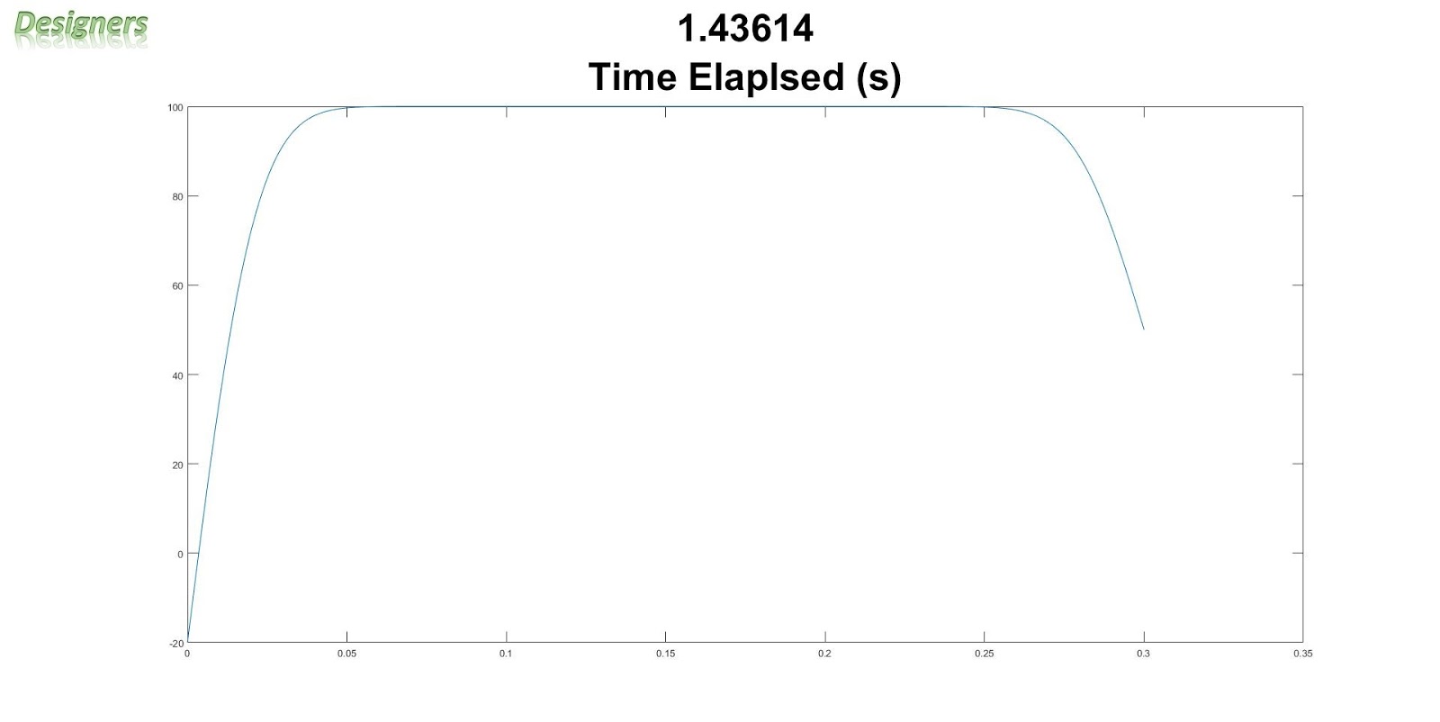
     It can be seen from Fig. 3-4 that time taken by the steady-state simulation to converge is on average 42.37% less that the transient analysis.  The steady-state analysis takes considerably less time to give a solution then a transient analysis.

 

Fig. 3, Solution time.

 

Fig. 4, Solution time.

 

Thank you for reading. If you would like to collaborate on research projects, please reach out.

1D Transient Diffusion (MATLAB code)

clear; clc;% clear the screen and memory

Nx=500; %number of space nodes

Nt=10000; %number of time nodes

Lx=0.3; %length of space (m)

Lt=10; %length of physical time (s)

dx=Lx/(Nx-1); %grid spacing

dt=Lt/(Nt-1); %time step

c=0.000097; %speed of wave (constant)

a=c*dt/dx.^2;

u=100*ones(Nx,1); %initialization of matrix for the property under investigation

x=zeros(Nx,1); %initialization of space

for i=1:Nx-1 %space loop

    x(i+1)=x(i)+dx;

end

u(1)=-20; %boundary condition

u(Nx)=50; %boundary condition

for t=0:dt:Lt %time loop

    un=u; %u(i,t)

    for i=2:Nx-1 %solution loop, backward in space forward in time

        u(i)=((1-2*a)*un(i))+a*(un(i+1)+un(i-1)); %discretized equation, u(i,t+1)

    end

    plot(x,u) %plotting

    title({t;'Time Elaplsed (s)'},'FontSize',38.5);

    pause(0.001)

end