High Camber Wing CFD Simulation

     This post is about the numerical simulation of a high camber, large aspect ratio wing. The wing had an aspect ratio of 5:1. The Reynolds number of flow was 500,000. The wing was at an angle of attack of zero degree. The aero-foil employed had a cross section of NACA 9410.

     The software employed was Flow Simulation Premium. A Cartesian mesh was created using the immersed boundary method. The mesh had 581,005 cells. Among those 581,005 cells, 55,882 were at the solid-fluid boundary. A time step of ~0.00528167 s was employed*. The domain was large enough to accurately trace the flow around the wing without any numerical or reversed flow errors. The software employs κ-ε turbulence model with damping functions, SIMPLE-R (modified) as the numerical algorithm and second order upwind and central approximations as the spatial discretization schemes for the convective fluxes and diffusive terms. The time derivatives are approximated with an implicit first-order Euler scheme.

     The mesh is shown in Fig. 1. The four layers of different mesh density are also visible in Fig. 1, the mesh is refined near the wing surface using a mesh control. The velocity around the wing section is shown in Fig. 2, using a cut plot at  the center of the wing. In Fig. 2, the wing body is super imposed by pressure plot. The velocity vectors showing the direction of flow are superimposed on both the wing body and the velocity cut plot.

Fig. 1, The computational domain.

Fig. 2, The velocity and pressure plots.

     The results of the simulation was validated against the results from XFLR5 software. XFLR5 predicted slightly higher lift and slightly less drag on the wing for same boundary conditions because the XFLR5 simulations were inviscid.

     Thank you for reading. If you would like to contribute to the research, both financially and scientifically, please feel free to reach out.

     *Time step is averaged because of the fact that a smaller time step was employed at the start of the numerical simulation.

Improvement of the Volume Flow Rate Through a Blower Fan

     In this post, an improvement in the volume flow rate through the blower fan assembly made are presented. The only thing changed in the blower fan was the cross section of the fan blades. In the previous version, the blade cross section resembled a flat plate with fillets at the leading edge. The trailing edge in the previous design was blunt. In the modified design, there aero-foils were selected, namely NACA 9410, NACA 9420 and the NACA 9430. All the other parameters were kept the same to the previous case. The CAD models of the modified fan blades are shown in Fig. 1.

Fig. 1, Fan blade geometries.

     The velocity contours are shown in Fig. 2 while the pressure contours are shown in Fig. 3, super imposed with velocity vectors and the computational mesh. The volume flow rate was the most for the fan with blades having cross-section of NACA 9410 aero-foil, followed by the fan with blades having cross-section of NACA 9420 and the NACA 9430 cross sections, respectively.

Fig. 2, Pressure contours. Row 1, L-R; fan with the NACA 9430 and NACA 9420 cross sections. Row 2, fan with NACA 9410 cross sections.

Fig. 3, Velocity contours. Row 1, L-R; fan with the NACA 9430 and NACA 9420 cross sections. Row 2, fan with NACA 9410 cross sections.

     Thank you for reading. If you would like to collaborate, both scientifically and financially, on research projects, please reach out.

Computational Fluid Dynamics Analysis of a Blower/Centrifugal Fan: Update 01

     In this post the results from a CFD analysis of a blower fan are presented. The fan had a diameter of 66 mm and a height of 12.57 mm. The fan's rotational velocity was at 10,000 rpm. The CAD model is shown in Fig. 1.

Fig. 1, CAD Assembly of the Blower Fan.

     The simulations were completed in SolidWorks Flow Simulation Premium code. The code employs immersed boundary method to create a Cartesian mesh. The sliding mesh feature was employed to simulate the rotation of the fan at atmospheric conditions. The code employs κ-ε model with Two-Scales Wall Functions approach as the turbulence model. The numerical algorithm implemented is the SIMPLE-R, modified. The second-order upwind discretization scheme is used to approximate the convective fluxes while the diffusive terms are approximated using the central differencing scheme. The time derivatives are approximated with an implicit first-order Euler scheme.

     The numerical model for the fan had 816,994 cells of which 209,421 cells were at the solid-fluid interface. Two mesh controls were employed to refine the mesh near the blades of the fan and at the boundary of the stationery and the rotating domains. The results were indeed, mesh independent. Due to the fact that this was an internal flow problem, domain independence test was not applicable. The mesh and the computational domain is shown in Fig. 2. The curved teal arrow represents the direction of rotation of the fan. The blue arrows represent the pressure boundary conditions at the inlet and at the outlet of the fan assembly. The straight teal arrow represents the force of gravity (the arrow is inverted).

Fig. 2, The mesh and the computational domain.

     The pressure and velocity plots are shown in Fig. 3-4.

Fig. 3, Pressure contours.

Fig. 4, Velocity contour

     Thank you very much for reading. If you would like to collaborate on research projects or want a tutorial for the setup of the numerical simulations such as this one, please reach out.

Update 01

     CAD files are available here.

Computational Fluid Dynamics Analysis of a Symmetrical Wing, Update 01

     This post is about the computational fluid dynamics analysis of a wing. The wing analyzed employed the NACA 0021 section throughout. The wing had a span of 4 m and a chord length of 1 m. The Reynolds number was kept at 3,000,000. The software employed was SolidWorks Flow Simulation Premium.

     The mesh had a total of 385,064 cells of which 84,826 cells were in contact with the wing surface, as shown in Fig. 1. The results are, indeed, mesh independent. Mesh controls were employed to refine the mesh near the wing surface. The computational domain employed was of cylindrical shape.

 

Fig. 1, The computational mesh around the wing.

 

     The velocity variation at various angles of attack around the wing cross-section is shown in Fig. 3 while the pressure variation on the wing surface is shown in Fig. 4. The results were validated against experiments conducted by [1].

 

Fig. 2, Velocity variation around the wing at 0-25 degree AOA, 5 degree increments.

 

Fig. 3, Pressure variation at the wing surface at 0-25 degree AOA, 5 degree increments.

     The purpose of this blog is maintain my online portfolio. I did this analysis because I realized I haven't written anything of this nature before. All of my previous simulations and/or blog entries were from the propulsion, renewable energy and turbo-machinery areas.
 

     Update 01

     CAD files are available here.

 

    
     Thank you for reading. If you would like to collaborate on research projects, please feel free to contact.

     [1] Fernando A. Rocha, Adson A. de Paula, Marcos d. Sousa, André V. Cavalieri, and Vitor G. Kleine, "Lift enhancement by wavy leading edges at Reynolds numbers between 700,000 and 3,000,000," Proceedings of the 2018 Applied Aerodynamics Conference, AIAA AVIATION Forum, Atlanta, GA, 2018.

     https://doi.org/10.2514/6.2018-3816

SolidWorks Flow Simulation: Internal Variable Velocity Inlet Boundary Condition

     This post is about an internal computational fluid dynamics simulation. The Simulation was performed in a pipe with a diameter of 1 in. The length of the inlet was 8 in away from the intersection. The two outlets were 4 in away from the intersection and were at an angle of 120° from the inlet, respectively. The flow entered the pipe in pulses with a period of 0.2 s. The peak velocity was at 2 m/s and the minimum velocity was kept at 0 m/s. This simulation setup can be analogous to the opening/closing of an IC engine valve simulation or simulation of cardiovascular systems etc.

     The part used in the simulation and the simulation setup is available here, as shown in Fig. 1.

Fig. 1, Part geometry.

 

     The mesh is shown in Fig. 2. The simulation assumed 2D simplification, to save time and computational resources. The mesh had a total of 15,512 cells. A simulation time step of 0.00625 s was employed.

 

Fig. 2, The computational mesh.

 

     The velocity profile at 0.9 s is shown in Fig. 3.

 

Fig. 3, Velocity Streamlines colored by velocity magnitude, superimposed by velocity vectors.

 

     An animation of the results is shown below. The results are, indeed, mesh and time independent.

 

 

     Thank you for reading. Reach out to collaborate in research projects.

Computational Fluid Dynamics (CFD) Analysis of a Horizontal Axis Tidal Turbine (Update 01)

     In this post, the results of numerical simulations carried out on a three-blade horizontal-axis tidal turbine blades are made available. These simulations are a part of larger project relating to a horizontal-axis tidal turbine.

 

     The turbine under investigation had a diameter of 4 m. The aero-foils employed include the NACA 4424 (chord length 0.25 m), NACA 4420 (chord length 0.2312 m), NACA 4418 (chord length 0.2126 m), NACA 4417 (chord length 0.1938 m), NACA 4416 (chord length 0.175 m), NACA 4415 (chord length 0.1562 m), NACA 4414 (chord length 0.1376 m), NACA 4413 (chord length 0.1188 m) and the NACA 4412 (chord length 0.1 m) at a distance of 0.4 m, 0.6 m, 0.8 m, 1 m, 1.2 m, 1.4 m, 1.6 m, 1.8 m, 2 m from the blade root, respectively [1].

 

     The numerical simulations were carried out on SolidWorks Flow Simulation Premium software. The software employs κ-ε turbulence model with damping functions, SIMPLE-R (modified) as the numerical algorithm and second order upwind and central approximations as the spatial discretization schemes for the convective fluxes and diffusive terms. The time derivatives are approximated with an implicit first-order Euler scheme. To predict turbulent flows, the Favre-averaged Navier-Stokes equations are used. The software employs a Cartesian mesh which is created using the immersed boundary method.

 

     The simulations were carried out using the Local rotating region(s) (Sliding) technique. The mesh had a total of 589,763 cells. 132,045 cells were at the turbine blade-rotating region boundary. While the process of mesh generation, a mesh control was employed to refine the mesh near the turbine blades and at the boundary of the rotating region and the stationery computational domain. To refine the mesh for the mesh independent test, the curvature level was increased i.e. the mesh in the areas of interest was refined by a factor of 8. As a result, the refined mesh had a total of 916,577 cells. A total of 221,978 were present around the turbine blade. The computational mesh around the turbine blade is shown in Fig. 1. The refined mesh in the areas of high gradients is also clearly visible. The computational domain had dimensions of 2D x 2D x 2.4D, where D is the diameter of the turbine. The dimensions for the computational domain resemble to those in [2].

     Fig. 2 shows computational domain around the turbine blades. In Fig. 2, the curved teal arrow represents the direction of rotation of the turbine. The green arrows represent the respective co-ordinate directions. The brown arrow represents the direction of the force of gravity. The blue arrow represents the direction of the fluid velocity. The circular disc represents the rotating region.

 

Fig. 1, The computational mesh.

    

Fig. 2, The computational domain and the orientation of the boundary conditions.

 

     The simulations were carried out for a total of 5 tip-speed ratios for the turbine ranging from 2 to 10. The fluid; water, velocity was set at 2 m/s. The results are indeed, mesh independent. The mesh independence test was conducted on the design point of the turbine i.e. at the TSR of 6. The plot between the turbine tip-speed ratio; TSR, and the co-efficient of power is shown in Fig. 3. It can be clearly seen from Fig. 3 that the results are in close agreement with the results from [1, 3]. The CFD results from both studies are lower then the BEM, Blade-Element Momentum, results because the three-dimensional effects are not considered while implementing the BEM method.

 

Fig. 3, Turbine efficiency plot.

 

     Fig. 4 shows velocity streamlines colored by velocity magnitude, both of these features are drawn relative to the rotating reference frame, around the turbine blade cross-section at various tip-speed ratios. It can be seen from Fig. 4 that the turbine stalls at TSR of 2 due to a large positive angle of attack. It can also be seen that as the TSR increases, the angle of attack on the blade decreases, it is because of this reason that the power output from the turbine increases.

 

 

Fig. 4, Row 1, L-R; TSR of 2 and 4. Row 2, L-R; TSR of 6 and 8. Row 3, TSR of 10.

 

     Thank you for reading. If you would like to collaborate with research projects, please reach out.

     [1] Binoe E. Abuan, and Robert J. Howell, "The Influence of Unsteady Flow to the Performance of a Horizontal Axis Tidal Turbine," Proceedings of the World Congress on Engineering. London, 2018.

     [2] Ibrahim, I. H., and T. H. New, "A numerical study on the effects of leading-edge modifications upon propeller flow characteristics," Proceedings of Ninth International Symposium on Turbulence and Shear Flow Phenomena. Melbourne, 2015.
     [3] Bahaj, A., Batten, W., & McCann, J. (2007). Experimental verifications of numerical predictions for the hydrodynamic performance of horizontal axis marine current turbines. Renewable Energy, 2479-2490.

Update 01:

     CFD post processing added. One more TSR simulated.

Steady-State VS Transient Propeller Numerical Simulation Comparison

     This post is about the comparison between steady-state and transient computational fluid dynamics analysis of two different propellers. The propellers under investigation are 11x7 and 11x4.7 propellers. The first number in the propeller nomenclature is the propeller diameter and the second number represents the propeller pitch, both parameters are in inch. The transient analysis was carried out using the sliding mesh technique while the steady-state results were obtained by the local rotating region-averaging method. For details about 11x7 propeller click here, for the details about 11x4.7 propeller, click here.

 

     As expected, the propeller efficiencies of transient and steady-state analysis are within 0.9% of each other, as shown in Fig. 1-2. Therefore, it is advised to simulate propellers and horizontal axis wind turbines using the steady-state technique as long as no time-dependent boundary conditions are employed.

 

Fig. 1, Propeller efficiency plot.

  

 Fig. 2, Propeller efficiency plot.

 

     It can be seen from Fig. 3-4 that time taken by the steady-state simulation to converge is on average 42.37% less that the transient analysis.  The steady-state analysis takes considerably less time to give a solution then a transient analysis.

 

Fig. 3, Solution time.

 

Fig. 4, Solution time.

 

Thank you for reading. If you would like to collaborate on research projects, please reach out.

SolidWorks Flow Simulation Premium: Propeller/Horizontal Axis Wind Turbine CFD Tutorial

The tutorial is in the attached video. Analysis such as: 11x7 Aeronautic Propeller Characteristics, 11x4.7 Aeronautic Propeller Characteristics and Wind Turbine SolidWorks Flow Simulation Premium Computational Fluid Dynamics are setup using the same method.

11x7 Aeronautic Propeller Characteristics (Using CFD) (Verified and Validated) (Update 02)

     This post presents the results from an aeronautic propeller CFD analysis.

    
     An 11x7 propeller was modelled using SolidWorks CAD package using the geometry from [1]. The simulations were run at two different rotational velocities and each rotational velocity was simulated at three advance ratios. The mesh for the 3,000 RPM rotational velocity had 213,205 total cells among which 24,048 cells were at the solid fluid boundary. While, the mesh for the 5,000 RPM rotational velocity had 369,963 total cells among which 68,594 cells were at the solid fluid boundary. A mesh control was employed to refine the mesh near the propeller geometry and at the boundary of the rotating region and the stationery domain for all of the cases simulated. This was done to ensure accuracy of the results was within an acceptable range. The results of the numerical simulations are plotted along with the experimental results [1] in Fig. 1.

Fig. 1 J= Advance Ratio, η_prop = propeller efficiency

     It can be seen from Fig. 1 that the trends for the propeller efficiency are in agreement with the experimental results. To increase the mesh density for the mesh independence test, the number of cells in  each of the respective co-ordinate directions was increased by a factor of 1.1. The mesh is shown in the Fig. 2.

Fig. 2 The computational mesh around the propeller.

     The computational domain size was at 2D x 2D x 2.4D, D being the propeller diameter, as shown in Fig. 3. In Fig. 3, the curved teal arrow represents the direction of rotation of the sliding mesh. The blue arrow represents the direction of free stream velocity while the brown arrow represents the force of gravity.

 Fig. 3 The computational domain.

Fig. 4 The pressure distribution and the velocity vectors around the propeller.

     The CAD model files and the simulation setup files for the numerical analysis are available here.

     Thank you for reading. If you'd like to collaborate on research projects, please reach out.

[1] Brandt, J. B., & Selig, M. S., “Propeller Performance Data at Low Reynolds Numbers,” 49th AIAA Aerospace Sciences Meeting, AIAA Paper 2011-1255, Orlando, FL, 2011.

doi.org/10.2514/6.2011-1255

 

Update 01

     Results from the mesh independent study are now available.

Update 02

     CAD model files are now uploaded. The CFD simulation setup files are also included.

11x4.7 Aeronautic Propeller Characteristics (Using CFD) (Verified and Validated) (Update 02)

     This post presents the results from an aeronautic propeller CFD analysis.

     An 11x4.7 propeller was modelled using SolidWorks CAD package using the geometry from [1]. The simulations were run at two different rotational velocities and each rotational velocity was simulated at three advance ratios. The mesh for the 3,000 RPM rotational velocity had 206,184 total cells among which 22,103 cells were at the solid fluid boundary. While, the mesh for the 6,000 RPM rotational velocity had 357,300 total cells among which 64,012 cells were at the solid fluid boundary. A mesh control was employed to refine the mesh near the propeller geometry and at the boundary of the rotating region and the stationery domain for all of the cases simulated. This was done to ensure accuracy of the results was within an acceptable range. The results of the numerical simulations are plotted along with the experimental results [1] in Fig. 1.

Fig. 1 J= Advance Ratio, η_prop = propeller efficiency

 

     It can be seen from Fig. 1 that the trends for the propeller efficiency are in agreement with the experimental results. The fine mesh had the number of cells in each of the respective co-ordinate directions increased by a factor of 1.1. The mesh is shown in the Fig. 2.

 

Fig. 2 The computational mesh around the propeller.

 

     The computational domain size was at 2D x 2D x 2.4D, D being the propeller diameter, as shown in Fig. 3. In Fig. 3, the curved teal arrow represents the direction of rotation of the sliding mesh. The blue arrow represents the direction of free stream velocity while the brown arrow represents the force of gravity.

Fig. 3 The computational domain.

Fig. 4 The pressure distribution and the velocity vectors around the propeller.

     The CAD model and numerical simulation setup files are available here.

 

     Thank you for reading. If you'd like to collaborate on research projects, please reach out.

     [1] Brandt, J. B., & Selig, M. S., “Propeller Performance Data at Low Reynolds Numbers,” 49th AIAA Aerospace Sciences Meeting, AIAA Paper 2011-1255, Orlando, FL, 2011.

doi.org/10.2514/6.2011-1255

 

Update 01

     Mesh independent test results are now available.

 

Update 02

     CAD files for the propeller including the CFD analysis setup are now available.

Desktop Computer Part List (Summer 2018-Pakistan Market)

     At the time of writing, 1 USD = Rs. 121.936. The prices mentioned in this post are based on the local market prices of computer components in Pakistan. Please remember that, prices vary from city-to-city within the country and shop-to-shop within a city. This is the reason why a price range is mentioned.

CPUs

     Intel Core i7-8700 for Rs. 41,500-Rs. 43,500. Top of the line processor from Intel. Always prefer a Core i7 or a Core i9 processor.

     Intel Core i5-8400 Processor Rs. 26,000-Rs. 28,000. Only buy this processor if there is a budget constraint.

Motherboard

     Gigabyte Z370 AORUS Gaming 3 for Rs. 21,200-Rs. 21,500. This motherboard has many USB ports and also comes equipped with a USB type-C port and M.2 slots etc. for future proofing.

Storage

     WD Blue 500GB Solid State Drive - WDS500G1B0A for Rs. 16,500-Rs. 17,500. Please do not buy a hard drive with rotating mechanism, it's 2018! When later in the year the SSD's prices go down, probably around November-December 2018, then buy another ~500 GB SSD. Do not waste money on a legacy hard drive.

Memory

     Corsair Vengeance LPX 16GB (1x16GB) DDR4 DRAM 3000MHz Rs. 25,800-Rs. 32,000. Please do not buy two sticks of 8 GB each. Save the remaining memory slots for future upgrading. Memory prices will fall significantly in October-November 2018 once the Chinese memory plants become operational. Don't fall for the shop keepers trickery. A common ploy employed by shopkeepers is that 1x16GB memory modules don't work in single channel mode for the 2400 MHz+ modules. It works perfectly well.

Casing

     Corsair Carbide Series® 100R Mid-Tower Case Rs.6,650-Rs. 7,500. This is the best option, really. Don't waste money on casing, it's just a box.

Power Supply

     Corsair VS550 - 550 Watt Power Supply Rs.5,800 -Rs. 6,000. A 550 Watt power supply for an i7 8700 CPU, 4 sticks of 1x16GB DDR4 memory modules, 1 SSD and up to a GTX 1x70 level graphic cards without any over clocking and 16 hours per day usage will be enough. May be this power supply will even be enough for GTX 1180 graphic card, as the graphic card chips are becoming more and more energy efficient. Yet again, do not fall for the shop keepers ploys.

Graphic Card

     Wait for the graphic new graphic cards from NVidia. The new cards are just around the corner. Local shops in Pakistan are selling 2 year old graphic cards, the GTX 10 series, at much inflated prices as compared to the rest of the world.

Conclusion

     This system will last at least 5 years, in terms of gaming with a GTX 1x70 level graphics card. It will even perform well for 10+ years if you keep upgrading it and take care of it cooling wise. Upgrade to a PCIe-NVMe SSD down the road when the prices drop, add more memory and update the graphic card every 5 years etc. Currently, the system will cost anywhere between Rs. 118,000 -Rs. 128,000, depending on you city and the shop, with an i7 processor.

     If you'd like to collaborate on research projects, please reach out. Thank you for reading.

Marine Propeller Characteristics (Using CFD) (Verified and Validated)

     This post presents the results from a marine propeller CFD analysis. The key thing about this CFD analysis was that the propeller efficiency obtained was within 7% of the experimental results, by using only 112,081 total cells in the computational mesh, of these cells, 21,915 cells were at the solid fluid boundary. The results are, indeed, mesh independent. The software employed was Flow Simulation Premium. The results of the numerical simulations are plotted along with the experimental results in Fig. 1.

Fig. 1 K_T = coefficient of thrust, 10K_Q = coefficient of torque multiplied by a factor of 10, η_prop = propeller efficiency

 

     It can be seen from Fig. 1 that the trends for the thrust and the torque coefficients and the propeller efficiency are in agreement with the experimental results. The experimental data was taken from here. The flow conditions were following. The propeller diameter was at 0.254 m. Propeller rotational velocity was at 15 rev/s. The propeller inclination angle was at 12°. Fluid considered was water. To change the advance ratio, fluid flow velocity was altered. The computational domain size was at 2D x 2D x 3.2D, D being the propeller diameter, as shown in Fig. 3. The mesh is shown in the Fig. 2.

Fig. 2 The computational mesh around the propeller.

 

Fig. 3 The computational domain.

 

     In Fig. 3, the curved teal arrow represents the direction of rotation of the sliding mesh. The blue arrow represents the direction of free stream velocity while the brown arrow represents the force of gravity. The Pressure distribution on the propeller blades and the velocity streamlines are shown in Fig. 4. The streamlines were drawn using line integral convolution, relative to the rotating frame of reference.

 

Fig. 4 The pressure distribution and the velocity profile around the propeller.

 

     If you'd like to collaborate on research projects, please reach out. Thank you for reading.

Comparison of VAWT Blade Designs (Leading-Edge Tubercle, Leading and Trailing-Edge Tubercle, Unmodified) (Update 05)

Numerical simulations were run on SolidWorks Flow Simulation Premium (model files are available here) software to compare the torque characterizes of three distinct vertical-axis wind turbine blade designs shown in Fig. 1. The torque characteristics are shown in Fig. 2.

This publication was used to verify and validate the numerical methodology. The results were within 8% of the publication's results at the design point of TSR of 1.2 at 90 RPM and 7.85 m/s wind speed. The dimensions of the turbine, the  blades and the cross section used are mentioned in the publication.

Fig. 1. Top Row, L-R: VAWT with blades having tubercles at the leading edge (ten tubercles per blade span, configuration name 10T), VAWT with blades having tubercles at both the leading and the trailing edge (ten tubercles per blade span). Bottom Row, VAWT with blades having no modifications.

It is clear from the Fig. 2 that the baseline design provides the most stable torque. On average the turbine with no modifications on the blades produced 5.31 Nm torque in one complete rotation, while the turbine with tubercles at the leading edge only, produced 5.20 Nm torque. The turbine with tubercles added to both the leading and the trailing edge produced 5.09 Nm torque in one complete rotation.

The peak torque was maximum for the turbine with the leading edge tubercles, followed by the turbine with the tubercles added to both the leading and the trailing edge of the turbine blades and the turbine with no modifications on the blades at 21.59 Nm, 21.45 Nm and 20.58 Nm respectively.

Fig. 2. Top Row, L-R: Torque curves for VAWT with blades having tubercles at the leading edge, Torque curves for VAWT with blades having tubercles at both the leading and the trailing edge. Bottom Row, Torque curves for VAWT with blades having no modifications. Three colors denote each of the blades in the turbine.

CFD post processing will be added later (may be next week). The effect of leading edge tubercle geometry will be investigated next. The blade design with tubercles added to both the leading and the trailing edge will not be investigated further because it produced the lowest average torque and second highest peak torque.

Update 01:

Decreased the number of tubercles per unit length of the blade, i.e. made the wavelength of the tubercles longer, kept the sweep angle same. As a result, the average and peak torque decreased to 4.53 Nm, and 19.33 Nm, respectively. The figure is attached.

Fig. 3. T-B: Torque curves for VAWT with blades having large wavelength tubercles at the leading edge (five tubercles per blade span, configuration name 5T45). Three colors denote each of the blades in the turbine. Render of the blades.

Update 02:

Increased the number of tubercles per blade span, i.e. made the wavelength of the tubercles smaller, kept the sweep angle same. As a result, the average and peak torque increased to 5.80 Nm, and 23.36 Nm, respectively. The figure is attached.

Fig. 4. T-B: Torque curves for VAWT with blades having smaller wavelength tubercles at the leading edge (fifteen tubercles per blade span, configuration name 15T45). Three colors denote each of the blades in the turbine. Render of the blades.

Update 03:

Again, increased the number of tubercles per blade span, i.e. made the wavelength of the tubercles smaller, kept the sweep angle same. As a result, the average and peak torque increased to 6.1 Nm, and 24.12 Nm, respectively. The figure is attached.

Fig. 5. T-B: Torque curves for VAWT with blades having smaller wavelength tubercles at the leading edge (twenty tubercles per blade span, configuration name 20T45). Three colors denote each of the blades in the turbine. Render of the blades.

Update 04:

Once more, increased the number of tubercles per blade span, i.e. made the wavelength of the tubercles smaller, kept the sweep angle same. As a result, the average and peak torque increased to 6.42 Nm, and 24.63 Nm, respectively. The figure is attached.

Fig. 6. T-B: Torque curves for VAWT with blades having smaller wavelength tubercles at the leading edge (twenty-five tubercles per blade span, configuration name 25T45). Three colors denote each of the blades in the turbine. Render of the blades.

A table for the tubercle geometry is shown below.

Table 01, Tubercle Geometry

Configuration Name	Amplitude (m)	Wavelength (m)	Sweep Angle (°)
Baseline	0	0	0
5T45	0.12777778	0.25555556	45
10T45	0.06052632	0.12105263	45
15T45	0.03965517	0.07931034	45
20T45	0.02948718	0.05897436	45
25T45	0.02346939	0.04693878	45

It is evident from Table 2 that adding more tubercles to the wind turbine's blade causes an increase in both the peak and the average torque. But it is also clear from the Table 2 that the percentage difference in both the average and the peak torque from the previous configuration (less tubercles per blade span) decreases as the number of tubercles per blade span is increased. It appears to be converging to a value.

Table 02, Tubercle Efficiency

Configuration Name	Peak Torque (Nm)	Average Torque (Nm)	Percentage Difference in the Average Torque from the Previous Configuration	Percentage Difference in the Average Torque from then Baseline Configuration
Baseline	20.58	5.31	N/A	N/A
5T45	19.33	4.53	-17.22	-17.22
10T45	21.59	5.2	12.89	-2.12
15T45	23.36	5.8	10.35	8.45
20T45	24.12	6.1	4.92	12.95
25T45	24.63	6.42	4.98	17.29

I think the difference between both the peak and the average torque produced by 25T45 and 20T45 configuration is comparable, up next, a new sweep angle.

Update 05

Following are my publications relating to the subject of this post.

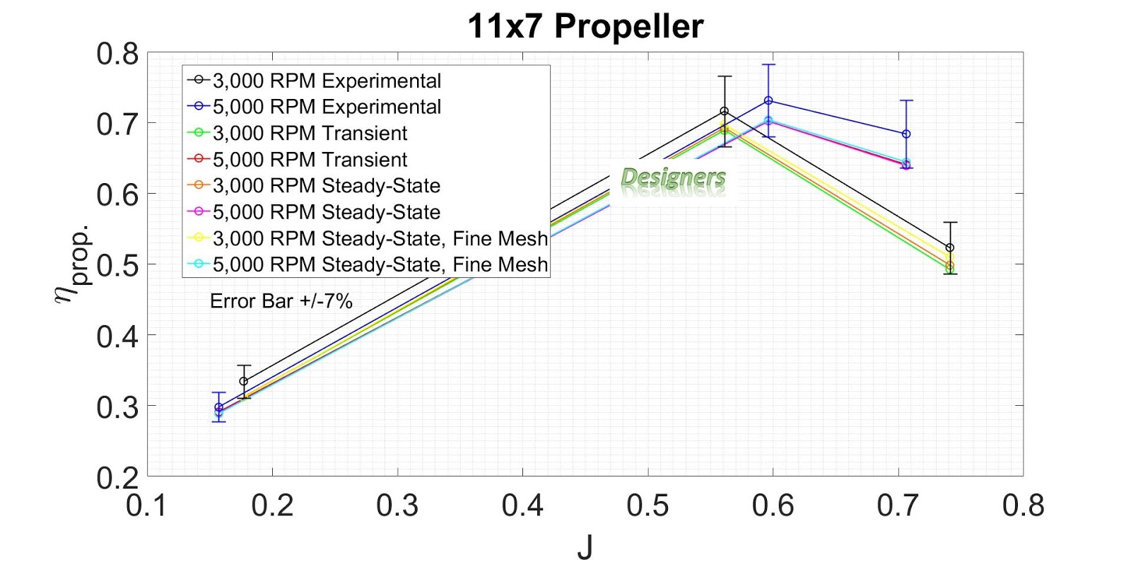
Butt, F.R., and Talha, T., "A Numerical Investigation of the Effect of Leading-Edge Tubercles on Propeller Performance," Journal of Aircraft. Vol. 56, No. 2 or No. 3, 2019, pp. XX. (Issue/page number(s) to assigned soon. Active DOI: https://arc.aiaa.org/doi/10.2514/1.C034845)

Butt, F.R., and Talha, T., "A Parametric Study of the Effect of the Leading-Edge Tubercles Geometry on the Performance of Aeronautic Propeller using Computational Fluid Dynamics (CFD)," Proceedings of the World Congress on Engineering, Vol. 2, Newswood Limited, Hong Kong, 2018, pp. 586-595, (active link: http://www.iaeng.org/publication/WCE2018/WCE2018_pp586-595.pdf).

Butt, F.R., and Talha, T., "Optimization of the Geometry and the Span-wise Positioning of the Leading-Edge Tubercles on a Helical Vertical-Axis Marine Turbine Blade ," AIAA Science and Technology Forum and Exposition 2019, Turbomachinery and Energy Systems, accepted for publication.

Thank you for reading.