Open - Source coded 3D Navier–Stokes equations in C++

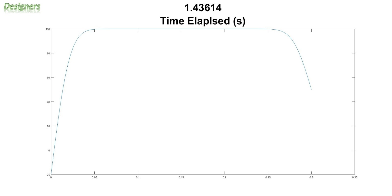
     Here are 3D Navier–Stokes equations configured for lid-driven cavity flow. The syntax is C++. The results from this code are shown in Fig. 1. From the pressure-Poisson equation, I removed mixed derivative terms to improve solution stability. 😆

p[i][j][k] = ((p[i+1][j][k] + p[i-1][j][k]) * h * h + (p[i][j+1][k] + p[i][j-1][k]) * h * h + (p[i][j][k+1] + p[i][j][k-1]) * h * h) / (2 * (h * h + h * h + h * h)) - h * h * h * h * h * h / (2 * (h * h + h * h + h * h)) * (rho * (1 / dt * ((u(i+1, j, k) - u(i-1, j, k)) / (2 * h) + (v(i, j+1, k) - v(i, j-1, k)) / (2 * h) + (w(i, j, k+1) - w(i, j, k-1)) / (2 * h))));

p[0][j][k] = p[1][j][k];

p[num_i - 1][j][k] = p[num_i - 2][j][k];

p[i][0][k] = p[i][1][k];

p[i][num_j - 1][k] = p[i][num_j - 2][k];

p[i][j][0] = p[i][j][1];

p[i][j][num_k - 1] = 0.0;

u[i][j][k] = u[i][j][k] - u[i][j][k] * dt / (2 * h) * (u[i+1][j][k] - u[i-1][j][k]) - v[i][j][k] * dt / (2 * h) * (u[i][j+1][k] - u[i][j-1][k]) - w[i][j][k] * dt / (2 * h) * (u[i][j][k+1] - u[i][j][k-1]) - dt / (2 * rho * h) * (p[i+1][j][k] - p[i-1][j][k]) + nu * (dt / (h * h) * (u[i+1][j][k] - 2 * u[i][j][k] + u[i-1][j][k]) + dt / (h * h) * (u[i][j+1] [k] - 2 * u[i][j][k] + u[i][j-1][k]) + dt / (h * h) * (u[i][j][k+1] - 2 * u[i][j][k] + u[i][j][k-1]));

u[0][j][k] = 0.0;

u[num_i - 1][j][k] = 0.0;

u[i][0][k] = 0.0;

u[i][num_j - 1][k] = 0.0;

u[i][j][0] = 0.0;

u[i][j][num_k - 1] = -Uinf;

v[i][j][k] = v[i][j][k] - u[i][j][k] * dt / (2 * h) * (v[i+1][j][k] - v[i-1][j][k]) - v[i][j][k] * dt / (2 * h) * (v[i][j+1][k] - v[i][j-1][k]) - w[i][j][k] * dt / (2 * h) * (v[i][j][k+1] - v[i][j][k-1]) - dt / (2 * rho * h) * (p[i][j+1][k] - p[i][j-1][k]) + nu * (dt / (h * h) * (v[i+1][j][k] - 2 * v[i][j][k] + v[i-1][j][k]) + dt / (h * h) * (v[i][j+1][k] - 2 * v[i][j][k] + v[i][j-1][k]) + dt / (h * h) * (v[i][j][k+1] - 2 * v[i][j][k] + v[i][j][k-1]));

v[0][j][k] = 0.0;

v[num_i - 1][j][k] = 0.0;

v[i][0][k] = 0.0;

v[i][num_j - 1][k] = 0.0;

v[i][j][0] = 0.0;

v[i][j][num_k - 1] = 0.0;

w[i][j][k] = w[i][j][k] - u[i][j][k] * dt / (2 * h) * (w[i+1][j][k] - w[i-1][j][k]) - v[i][j][k] * dt / (2 * h) * (w[i][j+1][k] - w[i][j-1][k]) - w[i][j][k] * dt / (2 * h) * (w[i][j][k+1] - w[i][j][k-1]) - dt / (2 * rho * h) * (p[i][j][k+1] - p[i][j][k-1]) + nu * (dt / (h * h) * (w[i+1][j][k] - 2 * w[i][j][k] + w[i-1][j][k]) + dt / (h * h) * (w[i][j+1][k] - 2 * w[i][j][k] + w[i][j-1][k]) + dt / (h * h) * (w[i][j][k+1] - 2 * w[i][j][k] + w[i][j][k-1]));

w[0][j][k] = 0.0;

w[num_i - 1][j][k] = 0.0;

w[i][0][k] = 0.0;

w[i][num_j - 1][k] = 0.0;

w[i][j][0] = 0.0;

w[i][j][num_k - 1] = 0.0;

Fig. 1, Velocity and pressure iso-surfaces

     Of course constants need to be defined, such as grid spacing in space and time, density, kinematic viscosity. These equations have been validated, as you might have read and here already! Happy coding!

     If you want to hire me as your PhD student in the research projects related to turbo-machinery, aerodynamics, renewable energy, please reach out. Thank you very much for reading.

1D Transient Diffusion (MATLAB code)

clear; clc;% clear the screen and memory

Nx=500; %number of space nodes

Nt=10000; %number of time nodes

Lx=0.3; %length of space (m)

Lt=10; %length of physical time (s)

dx=Lx/(Nx-1); %grid spacing

dt=Lt/(Nt-1); %time step

c=0.000097; %speed of wave (constant)

a=c*dt/dx.^2;

u=100*ones(Nx,1); %initialization of matrix for the property under investigation

x=zeros(Nx,1); %initialization of space

for i=1:Nx-1 %space loop

    x(i+1)=x(i)+dx;

end

u(1)=-20; %boundary condition

u(Nx)=50; %boundary condition

for t=0:dt:Lt %time loop

    un=u; %u(i,t)

    for i=2:Nx-1 %solution loop, backward in space forward in time

        u(i)=((1-2*a)*un(i))+a*(un(i+1)+un(i-1)); %discretized equation, u(i,t+1)

    end

    plot(x,u) %plotting

    title({t;'Time Elaplsed (s)'},'FontSize',38.5);

    pause(0.001)

end

 

 

SolidWorks Animation: Transient NREL Phase-VI Wind Turbine CFD Simulation [Validated]

     10 KW wind turbine CFD simulation using Flow Simulation Premium. Design points: 10 m/s wind speed, rotational velocity 7.5 rad/s.

     The rendered volume shows vorticity (curl of the velocity field). It is colored by dynamic pressure. Low pressure in the center of the helix shows very small wind speed.

     Power from the CFD analysis was 9,854.96 W while the experimental power is 10,000 W, a difference of only 1.45 %, that too by using only 693,141 cells in the mesh.

     Do you want me to make a tutorial about the simulation setup with SolidWorks Flow Simulation Premium?

Computational Fluid Dynamics: 1 Core VS 2 Cores VS 3 Cores VS 4 Cores. (SolidWorks Flow Simulation Premium)

Problem:
Lift and Drag calculation for a rectangular wing (0.5 m span x 0.15 m chord x uniform cross section of NACA 9410), at horizontal velocity of 10 km/h.

A very simple CFD problem (with 177250 cells) solved on a 4 core Haswell-DT, varying the number of CPU cores used each time; CPU times are as below:

Cores used            CPU time taken for solution (1 travel convergence)
1/4 core                 782 seconds (2.31x slower)
2/4 cores               468 seconds (1.38x slower)
3/4 cores               380 seconds (1.12x slower)
4/4 cores               339 seconds (1x)

Computational Fluid Dynamics: Finite Difference Approximations VS Analytical Differentiation (MATLAB)

Description of the Program

The program takes user input for the function of the variable ‘x’ e.g. x², sin(x), cos(x)/x² etc., the point on which the derivative is evaluated and initial and final grid sizes.

The program then calculates its first derivative analytically.

It then calculates finite difference approximations of the first derivative of order h, with point A unknown and the point A known, using various step sizes, with maximum and minimum step size enter by the user.

 It then calculates and plots the error between the exact value and the approximations of the first derivative.

Code along with Guidelines

clc; %clears the command window

 

%data input and analytical differentiation

 

syms x

fx=input('Enter the function of ''x'' to be differentiated '); %input a function like sin(x) or x.^4 + x.^3

clc; %clears the command window

fxp=(diff (fx,x)); %calculate the derivative analytically

x=input('Enter the point at which the derivative is to be evaluated '); %input the value at which the derivative to be evaluated

clc; %clears the command window

y=inline(fxp,'x'); %convert a statement in to a function so it can be evaluated at some point

z=y(x); %derivative evaluated at the point

 

 

dxmin=input('Enter the smallest value of increment ');

clc;

dxmax=input('Enter the largest value of increment ');

clc;

%finite difference approximation

for dx=dxmin:0.001:dxmax; %loop for different values of grid spacing, dx=h1

    a=1.5;

    h1=a*dx; %h2 in the problem sheet

    h2=(2*a*dx); %h3 in the problem sheet

   

    fc=cos(5+h2)/(5+h2).^2; %value of the function at point c

    fb=cos(5+h1)/(5+h1).^2; %of the function at point b

    fa=cos(5-dx)/(5-dx).^2; %of the function at point a

    fi=cos(x)/(x).^2; %of the function at point A

    fxpu=(fc+fb-(2*fa))/((2*dx)+h1+h2); %formulation with A unknown

    fxpa=(fc+fb+(2*fa)-(4*fi))/((-2*dx)+h1+h2); %formulation with A known

    hold on

    plot ((z-fxpa)/z,dx,'.k') %error plot for approximation with A known

    plot ((z-fxpu)/z,dx,'.r') %error plot for approximation with A unknown

end

%text editing

title('Plot Between Error VS Grid Spacing') %title of the graph

xlabel('Error from the Exact Value'); %x-axis label

ylabel('Step Size/Grid Spacing') %y-axis label

text(0.6, 0.9,'Red: Error plot for approximation with A unknown') %identification

text(0.6, 0.85,'Black: Error plot for approximation with A known') %identification

Calculation

Sample Problem

Command Window after running the code

At Step One

Enter the function of 'x' to be differentiated cos(x)/x.^2

At Step Two

Enter the point at which the derivative is to be evaluated 5

At Step Three

Enter the smallest value of increment 0.001

At Step Four

Enter the largest value of increment 1

Result

 

Observations and Recommendations

It was observed that the error in the finite difference approximation when the value of the function at point A is unknown is less as compared to the case where value of the function at point A is known.

In physical/real-world problems, the exact derivatives of the functions are not known, therefore the error values between the exact and the finite difference approximation cannot be calculated. As it is also observed that the error between finite difference approximation and the exact value of the derivative decreases as the step size decreases, it is advisable to use a step size of ~1/1000 to make a compromise between CPU/RAM usage, time taken to solve the problem and error.

References

[1] Le Moigne, "A Discrete Navier-Stokes Adjoint Method for Aerodynamic Optimization of Blended Wing-Body, Configurations", PhD thesis, Cranfield University, United Kingdom, 2002.
[2] J. Lee, C. S. Kim, C. Kim, O. H. Rho, and K. D. Lee, "Parallelized Design Optimization for Transonic Wings using Aerodynamic Sensitivity Analysis", AIAA Paper 2002-0264, 2002.
[3] E. J. Neilsen and W. K. Anderson, "Recent Improvements in Aerodynamic Design Optimization on Unstructured Meshes", AIAA Paper 2001-0596, 2001.
[4] 3D ONERA M6 Wing Validation, https://turbmodels.larc.nasa.gov/onerawingnumerics_val_sa.html.
Thank you for reading. If you would like to collaborate on research projects, please reach out.
Monday 26 March 2018