Aperiodic Aero-foil Kinematics

     This post is about a 2D NACA 0012 aero-foil undergoing forced aperiodic heaving. Heaving motion is achieved by the plot shown in Fig. 1. Plot within Fig. 1 represents position of airfoil at various time steps.

Fig. 1, The position of aero-foil

     The animation of the vorticity contours are shown in Fig. 2. The velocity, pressure and vorticity for aperiodic heaving is shown in Fig. 3. A comparison will be made with heaving later, if ever 😀. As far as aerodynamic forces are concerned, per-cycle C_{l, avg} is at 0.63 as compared to 0.0 for periodic heaving. C_{d, avg} aperiodic heaving is at 0.162 as compared to 0.085 for periodic heaving. Of course, this is done on a coarse mesh. If ever I write a paper about this... 😀

Fig. 2, Top Row, Aperiodic, periodic heaving airfoil 

     

Fig. 3, Top Row, L-R, Vorticity, pressure. Bottom Row, Velocity 

     If you want to collaborate on the research projects related to turbomachinery, aerodynamics, renewable energy, please reach out. Thank you very much for reading. 

Flapping Aerofoil For Propulsion

     This post is about a 2D NACA 0012 aerofoil undergoing forced flapping motion for propulsion purposes. Heaving motion is achieved by applying a vertical velocity on the aerofoil based on the Eqn. 1. Similarly the pitching motion is achieved by applying a rotational velocity, governed by Eqn. 2.

v_y = 2*π*f_h*H_o*sin(2*π*f_h*t)                                              Eqn. 1

ω = -2*π*f_h*ϑ*sin[(2*π*f_h*t) + 1.5708]                               Eqn. 2

     w.r.t. Eqn. 1-2 reduced frequency is defined as (2*π*f_h*H_o/U∞)), f_h is the frequency of oscillations, while ω, t and ϑ_o represent rotational velocity, instantaneous time and maximum pitching angle. H_o is the heaving amplitude and U∞ is the free stream velocity.

     The flapping motion is achieved by a combination of the heaving and pitching. In this particular simulation, the aerofoil is in the propulsion mode, meaning the feathering parameter χ is less in magnitude than 1.0. Feathering parameter is defined by Eqn. 3.

χ = ϑ/arctan(h0*2*π*f_h/U∞)                                  Eqn. 3

     The boundary conditions employed for the simulation are at Re 1,000, K = 1.41, H_o = aerofoil chord length, χ = 0.5489 and f_h = 0.003391 Hz. The animation of the pressure, vorticity and velocity contours is shown in Fig. 1.

Fig. 1, Flow animation, fluid flow direction is from left to right.

     The results of present simulation are compared with [1]. In terms of maximum lift, a maximum deviation of 5% is observed as compared to [1], as shown in Fig. 2. The maximum lift coefficient for available data is ~4.224 while the maximum lift coefficient from the present simulation is ~4.057. The average thrust produced is within 2% of [1]. Average thrust coefficient per cycle from [1] is 0.9957 while the result from present simulation reveals the thrust coefficient to be 1.0098.

Fig. 2, A comparison of coefficient of lift.

If you want to collaborate on the research projects related to turbo-machinery, aerodynamics, renewable energy, please reach out. Thank you very much for reading.

References

[1] https://doi.org/10.1017/jfm.2017.508

Steady-State VS Transient Propeller Numerical Simulation Comparison

     This post is about the comparison between steady-state and transient computational fluid dynamics analysis of two different propellers. The propellers under investigation are 11x7 and 11x4.7 propellers. The first number in the propeller nomenclature is the propeller diameter and the second number represents the propeller pitch, both parameters are in inch. The transient analysis was carried out using the sliding mesh technique while the steady-state results were obtained by the local rotating region-averaging method. For details about 11x7 propeller click here, for the details about 11x4.7 propeller, click here.

 

     As expected, the propeller efficiencies of transient and steady-state analysis are within 0.9% of each other, as shown in Fig. 1-2. Therefore, it is advised to simulate propellers and horizontal axis wind turbines using the steady-state technique as long as no time-dependent boundary conditions are employed.

 

Fig. 1, Propeller efficiency plot.

  

 Fig. 2, Propeller efficiency plot.

 

     It can be seen from Fig. 3-4 that time taken by the steady-state simulation to converge is on average 42.37% less that the transient analysis.  The steady-state analysis takes considerably less time to give a solution then a transient analysis.

 

Fig. 3, Solution time.

 

Fig. 4, Solution time.

 

Thank you for reading. If you would like to collaborate on research projects, please reach out.

11x7 Aeronautic Propeller Characteristics (Using CFD) (Verified and Validated) (Update 02)

     This post presents the results from an aeronautic propeller CFD analysis.

    
     An 11x7 propeller was modelled using SolidWorks CAD package using the geometry from [1]. The simulations were run at two different rotational velocities and each rotational velocity was simulated at three advance ratios. The mesh for the 3,000 RPM rotational velocity had 213,205 total cells among which 24,048 cells were at the solid fluid boundary. While, the mesh for the 5,000 RPM rotational velocity had 369,963 total cells among which 68,594 cells were at the solid fluid boundary. A mesh control was employed to refine the mesh near the propeller geometry and at the boundary of the rotating region and the stationery domain for all of the cases simulated. This was done to ensure accuracy of the results was within an acceptable range. The results of the numerical simulations are plotted along with the experimental results [1] in Fig. 1.

Fig. 1 J= Advance Ratio, η_prop = propeller efficiency

     It can be seen from Fig. 1 that the trends for the propeller efficiency are in agreement with the experimental results. To increase the mesh density for the mesh independence test, the number of cells in  each of the respective co-ordinate directions was increased by a factor of 1.1. The mesh is shown in the Fig. 2.

Fig. 2 The computational mesh around the propeller.

     The computational domain size was at 2D x 2D x 2.4D, D being the propeller diameter, as shown in Fig. 3. In Fig. 3, the curved teal arrow represents the direction of rotation of the sliding mesh. The blue arrow represents the direction of free stream velocity while the brown arrow represents the force of gravity.

 Fig. 3 The computational domain.

Fig. 4 The pressure distribution and the velocity vectors around the propeller.

     The CAD model files and the simulation setup files for the numerical analysis are available here.

     Thank you for reading. If you'd like to collaborate on research projects, please reach out.

[1] Brandt, J. B., & Selig, M. S., “Propeller Performance Data at Low Reynolds Numbers,” 49th AIAA Aerospace Sciences Meeting, AIAA Paper 2011-1255, Orlando, FL, 2011.

doi.org/10.2514/6.2011-1255

 

Update 01

     Results from the mesh independent study are now available.

Update 02

     CAD model files are now uploaded. The CFD simulation setup files are also included.

11x4.7 Aeronautic Propeller Characteristics (Using CFD) (Verified and Validated) (Update 02)

     This post presents the results from an aeronautic propeller CFD analysis.

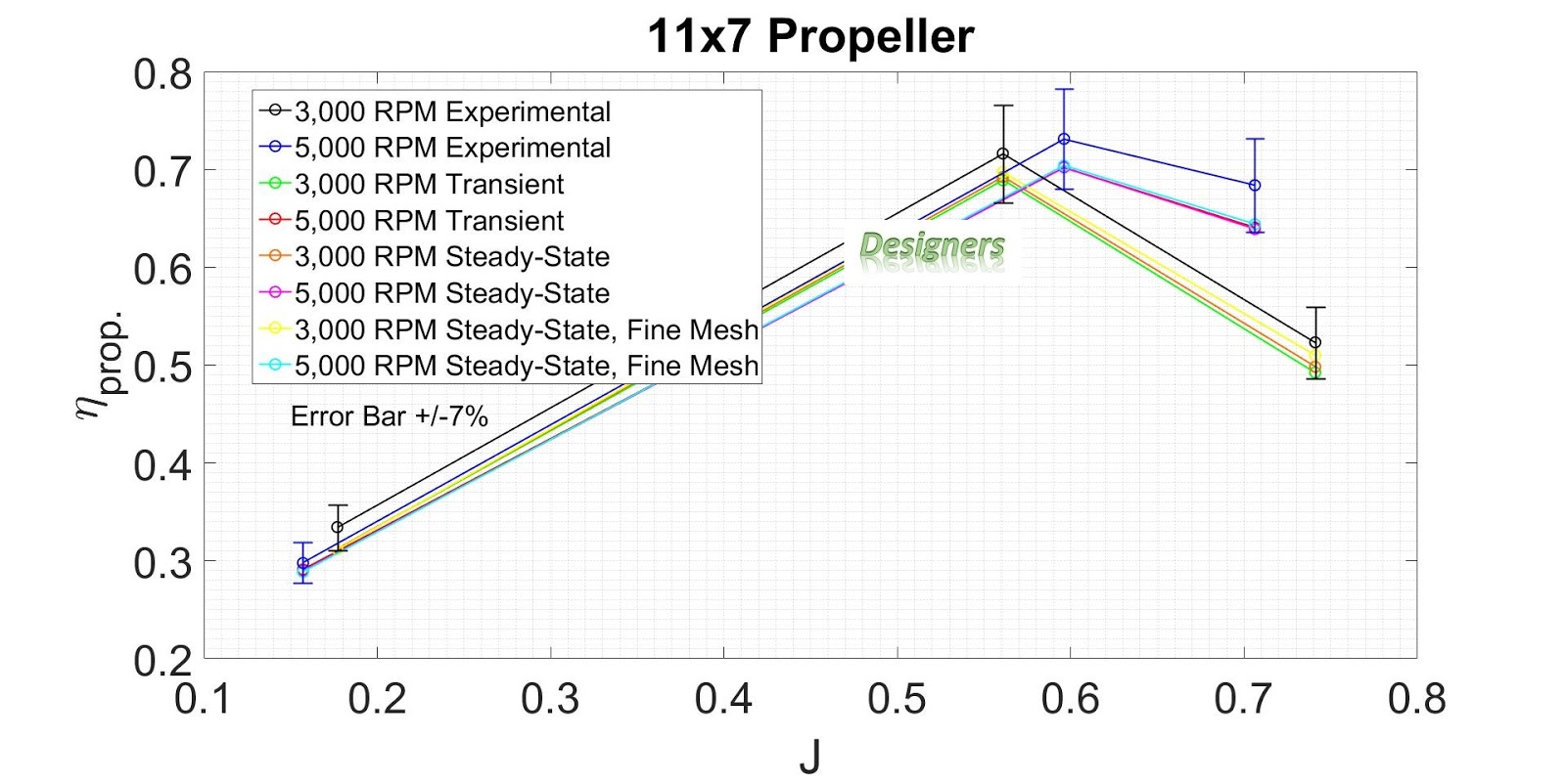
     An 11x4.7 propeller was modelled using SolidWorks CAD package using the geometry from [1]. The simulations were run at two different rotational velocities and each rotational velocity was simulated at three advance ratios. The mesh for the 3,000 RPM rotational velocity had 206,184 total cells among which 22,103 cells were at the solid fluid boundary. While, the mesh for the 6,000 RPM rotational velocity had 357,300 total cells among which 64,012 cells were at the solid fluid boundary. A mesh control was employed to refine the mesh near the propeller geometry and at the boundary of the rotating region and the stationery domain for all of the cases simulated. This was done to ensure accuracy of the results was within an acceptable range. The results of the numerical simulations are plotted along with the experimental results [1] in Fig. 1.

Fig. 1 J= Advance Ratio, η_prop = propeller efficiency

 

     It can be seen from Fig. 1 that the trends for the propeller efficiency are in agreement with the experimental results. The fine mesh had the number of cells in each of the respective co-ordinate directions increased by a factor of 1.1. The mesh is shown in the Fig. 2.

 

Fig. 2 The computational mesh around the propeller.

 

     The computational domain size was at 2D x 2D x 2.4D, D being the propeller diameter, as shown in Fig. 3. In Fig. 3, the curved teal arrow represents the direction of rotation of the sliding mesh. The blue arrow represents the direction of free stream velocity while the brown arrow represents the force of gravity.

Fig. 3 The computational domain.

Fig. 4 The pressure distribution and the velocity vectors around the propeller.

     The CAD model and numerical simulation setup files are available here.

 

     Thank you for reading. If you'd like to collaborate on research projects, please reach out.

     [1] Brandt, J. B., & Selig, M. S., “Propeller Performance Data at Low Reynolds Numbers,” 49th AIAA Aerospace Sciences Meeting, AIAA Paper 2011-1255, Orlando, FL, 2011.

doi.org/10.2514/6.2011-1255

 

Update 01

     Mesh independent test results are now available.

 

Update 02

     CAD files for the propeller including the CFD analysis setup are now available.

Marine Propeller Characteristics (Using CFD) (Verified and Validated)

     This post presents the results from a marine propeller CFD analysis. The key thing about this CFD analysis was that the propeller efficiency obtained was within 7% of the experimental results, by using only 112,081 total cells in the computational mesh, of these cells, 21,915 cells were at the solid fluid boundary. The results are, indeed, mesh independent. The software employed was Flow Simulation Premium. The results of the numerical simulations are plotted along with the experimental results in Fig. 1.

Fig. 1 K_T = coefficient of thrust, 10K_Q = coefficient of torque multiplied by a factor of 10, η_prop = propeller efficiency

 

     It can be seen from Fig. 1 that the trends for the thrust and the torque coefficients and the propeller efficiency are in agreement with the experimental results. The experimental data was taken from here. The flow conditions were following. The propeller diameter was at 0.254 m. Propeller rotational velocity was at 15 rev/s. The propeller inclination angle was at 12°. Fluid considered was water. To change the advance ratio, fluid flow velocity was altered. The computational domain size was at 2D x 2D x 3.2D, D being the propeller diameter, as shown in Fig. 3. The mesh is shown in the Fig. 2.

Fig. 2 The computational mesh around the propeller.

 

Fig. 3 The computational domain.

 

     In Fig. 3, the curved teal arrow represents the direction of rotation of the sliding mesh. The blue arrow represents the direction of free stream velocity while the brown arrow represents the force of gravity. The Pressure distribution on the propeller blades and the velocity streamlines are shown in Fig. 4. The streamlines were drawn using line integral convolution, relative to the rotating frame of reference.

 

Fig. 4 The pressure distribution and the velocity profile around the propeller.

 

     If you'd like to collaborate on research projects, please reach out. Thank you for reading.