Executive transport aircraft with truss-braced wing (World's First)

     To explore large-er aspect ratio wings; one fine morning, I just thought it would be fun to put a truss-braced wing in a Piaggio P.180 "Avanti". The modified design CAD files are is available here. A comparison is shown in Fig. 1. I am too lazy to make 2 separate airplanes so I modified half of it so I can run a CFD analysis using one model and one mesh 🤣. A slight modification about which I will write later is the positioning of the flaps and ailerons. These are moved to the truss part from the main wing in the original design. The aspect ratio is of the truss-braced section is double the original. With a foldable wing, storage shouldn't be a problem?

Fig. 1, Row 1, L-R Top, bottom; Row 2, L-R front, back; Row 3 L-R, left, right views

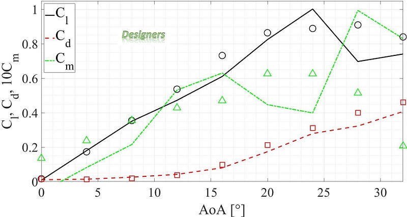
     Cruise conditions are taken from [1] i.e. ~12,500 m and ~163.6 m/s. The CFD mesh has 4,892,425 cells out of those, 449,732 are the the surface of the jet. I compare lift/drag of both halves. The modified section produces 36.15% more drag (force) as compared to the original design. The modified section however, produces 49% more lift (force) than the original design. L/D for truss-winged section is at 6.72 as compared to 6.14 for the original design. In terms of L/D, the truss-braced wing section produced 🥁 ... 9.45% more Lift/Drag. A resounding success 😁, I'd say. For validation of CFD, read this and this.

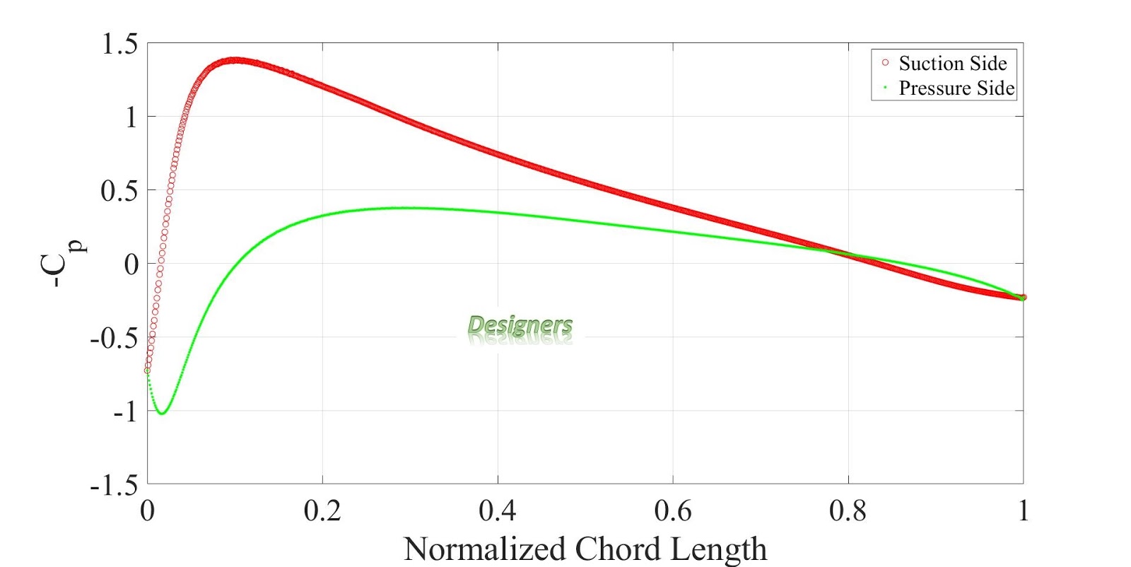
     Some post processing I did, is shown in Fig. 2. Velocity iso-lines with vectors are shown around the wings. Vorticity is shown in the wake of the jet(s). Tip vortex is smaller and less intense behind the truss-braced wing portion but there is another vortex where the truss meets with the main wing. In the main wing, for the trussed-braced portion; on the pressure side; the high pressure zones extend for a longer portion of the span in the span-wise direction as compared to the original design. Same is true for low pressure zones on the suction side of the main wing. Some day I will write a nice little paper and sent it to an AIAA conference, till then 𝌗.

Fig. 2, Colorful Fluid Dynamics 🌈

     Stream-wise vorticity is shown in Fig. 3. It is clear from Fig. 3 that the vorticity is less intense on the side with truss-braced wing as compared to the original design. Fig. 3 is colored by stream-wise velocity. The aircraft appears blue due to no slip condition.

Fig. 3, Some more Colorful Fluid Dynamics (CFD) 🌈

     Thank you for reading, if you would like to hire me as your master's / PhD student / post-doc / collaborate on research projects, please reach out! 😌

References

[1] "Operations Planning Guide". Business & Commercial Aviation. Aviation Week. May 2016. [https://web.archive.org/web/20160815060134/http://www.sellajet.com/adpages/BCA-2016.pdf]

Turbulent Fluid Structure Interaction (FSI) - Benchmark Case

     After weeks spent self-learning about this type of simulation and countless nights spent troubleshooting this complex problem, I am pleased to share results. 😇 This post is about the FSI analysis of the FSI-PfS-2a. A case designed by Dr. Breuer. The geometry is shown in Fig. 1. The geometry details are available in ref. [1]. The geometry is made in SolidWorks CAD package and then imported to ANSYS via .STEP file. FSI combines Computational Fluid Dynamics (CFD) and structural analysis, i.e. the Finite Element Method (FEM).

Fig. 1, The geometry

     A combination of ANSYS Fluent, Mechanical and System Coupling are used for the analysis. Fig. 2 shows post-processing animation from the simulation. The top left shows stress while the displacements of the material are shown in top right. Bottom left and right show fluid velocity and vorticity, respectively. The vorticity is plotted along the axis perpendicular to the both lift and drag forces. the image in the center of animation shows fluid pressure acting on the cylinder and plate. Stagnation pressure is observed to change with time.

Fig. 2, The animation

     The boundary conditions from Mechanical are shown in Fig. 3. The condition A refers to gravity at 9.8066 m/s2 while B refers to fixed-support condition applied to the edge touching the cylinder. Boundary condition C refers to the fluid-solid interface. It is at these regions forces and displacements are exchanged. The structural mesh has 180 elements and 1,156 nodes. It is to be noted that the fluid regions are not meshed in mechanical and vice-versa. Furthermore, the number of mesh elements is limited by the system memory. The steel and rubber portions are connected via 4 connections i.e. edge/edge and edge/face contacts. The unmarked regions within Fig. 3 (top) are made symmetric. The  steel and rubber are considered linear elastic. No external force is applied in mechanical so this case can also be called as a case of vortex-induced vibrations. The direct sparse FEM solver is used for the Structural-FSI simulation.

Fig. 3, The boundary conditions and mesh

     The CFD mesh is shown in Fig. 4. The mesh is created using sweep method. Refinements are applied in areas of interest, i.e. wake and around the structure, using bodies of influence. Moreover, inflation mesh for y+ of 7.55 is applied on the cylinder to properly capture the boundary layer. The FSI-CFD simulation is initialized with data from static transient analysis using k–ω SST DES turbulence model. The k–ω DES model is initialized using static steady-state k–ω SST model. The flow parameters include a velocity of 1.385 m/s [1] corresponding to a Reynolds number of 30,470. The mesh has 79,305 cells. The dynamic mesh is handled through remeshing and smoothing via the radial basis function. Water is taken as a fluid for this simulation, same as [1]. Symmetry is applied to the walls facing perpendicular to flow. Top and bottom walls of the structure are considered adiabatic and with no shear. The SIMPLE algorithm is used. 2nd order accurate discretization schemes are used.

Fig. 4, The computational domain and the mesh

     It should be noted that for this simulations only 20 mm section of the whole geometry is simulated. This is because of computational resources limitations. The simulations took ~12 hours to solve 0.268 s of physical time with 32 GB RAM and 6 core CPU. The mesh motion along with vorticity iso-surfaces are shown in Fig. 5.

Fig. 5, The mesh and vorticity animation

     Thank you for reading, if you would like to hire me as your PhD student / post-doc  / collaborate on projects, please reach out.

References

[1] A. Kalmbach and M. Breuer, "Experimental PIV/V3Vmeasurementsofvortex-induced fluid–structure interaction in turbulent flow—A new benchmark FSI-PfS-2a", Journal of Fluids and Structures, Vol. 42, pp 369–387, 2013

Datacenter Visualization (Verified and Validated)

     This simulation is done to create an aero-thermal digital twin of a datacenter using CFD. The details of datacenter are taken from [1]. The datacenter CAD model is shown in Fig. 1.

     The simulation employs κ − ε turbulence model with damping functions, SIMPLE-R (modified), as the numerical algorithm and second-order upwind and central approximations as the spatial discretization schemes for the convective fluxes and diffusive terms. The time derivatives are approximated with an implicit first-order Euler scheme. Flow simulation solves the Navier–Stokes equations, which are formulations of mass, momentum, and energy conservation laws for fluid flows. To predict turbulent flows, the Favre-averaged Navier–Stokes equations are used.

Fig. 1, Datacenter CAD

     A Cartesian mesh with octree refinement, cut-cell method and immersed boundary methods is used. Special mesh refinements are deployed in the areas of interest i.e. inlets and outlets and sharp edges of server racks and CRAH units to accurately capture aero-thermal gradients and vortices. The resulting computational mesh has 2,698,156 cells. The computational domain and mesh are shown in Fig. 2.

Fig. 2, Computational mesh and domain

     The results from the numerical analysis were compared with [1]. The results are in excellent agreement with previously published data. The animation in Fig. 3 shows thermal distribution inside datacenter using cut-plots. Fluid velocity distribution is also shown. The cut-plots are superimposed with streamlines and velocity vectors. These post processing features help identify hot-spots and recirculation zones. Design improvements can be made to reduce thee unwanted flow features. Within Fig. 3, Flow trajectories colored by air temperature are also shown. These show path the fluid takes between various inlets and outlets in the datacenter such as the CRAH system supply and return zones and inlets and outlets of servers. Fig. 4 shows various post processing tools available for diagnosing various issues from the aero-thermal perspective. These include iso-surfaces, cut-plots, flow trajectories and surface plots etc.

Fig. 3, The post processing animations

Fig. 4, The post processing images

     A comparison of the results from present simulations with previously published literature is shown in Fig. 5. it can be seen that out results are in close agreement with previously published numerical and experimental data [1]! The locations at which the data is extracted is shown in Fig. 6. Within Fig. 5, solid lines indicate present study, dashed lines indicate published numerical results and filled circles represent published experimental results.

Fig. 5, Comparison of results

Fig. 6, Location of data extraction

     If you want to collaborate on the research projects related to turbomachinery, aerodynamics, renewable energy, please reach out. Thank you very much for reading.

References

[1] Wibron, Emelie, Anna-Lena Ljung, and T. Staffan Lundström. 2018. "Computational Fluid Dynamics Modeling and Validating Experiments of Airflow in a Data Center" Energies 11, no. 3: 644. https://doi.org/10.3390/en11030644

DARPA Suboff Submarine CFD Simulation (Backed-up by Water Tunnel Data); Update 01: Water Level Simulations (Volume of Fluid)

      This post is about the CFD analysis of the DARPA Suboff at various speeds. The DARPA Suboff model is based on a generic submarine. The submarine geometry is shown in Fig. 1. The submarine in fully submerged in water. Refer to section "Update 01" for submarine sailing at the water level. The submarine geometry is available here. The geometry is made using equations from [1]. Machine Learning available here.

Fig. 1, DARPA Suboff submarine CAD

      The simulations are validated with published literature [2-4]. SolidWorks Flow Simulation Premium software is employed for the simulations. Fig. 2 shows results of drag force at various cruise speeds. It can be seen that the results are in close agreement with the published experimental / numerical data.

Fig. 2, Comparison of results

     The mesh has 656,714 cells in total. With 34,258 cells on the submarine surface. Special mesh refinements are added in the regions of interest i.e. regions with high gradients, the wake and on the control surfaces of the submarine. The mesh for is shown in Fig. 3.

Fig. 3, The mesh and computational domain

     The results from the CFD post processing are presented next. Velocity cut-plots showing velocity distribution and wake of the submarine, surface pressure distribution on the submarine and vorticity around and in the wake of the submarine are also shown in Fig. 4. Within Fig. 4, the black arrows represent the direction of on coming flow.

Fig. 4, The post processing

     Thank you for reading, If you would like to collaborate on projects, please reach out.

Update 01

     This section presents the results from a simulation using volume of fluid method. The water line is just below the sail of the submarine, as shown in Fig. 5. The iso-surfaces are shown in Fig. 6. The black arrows in both Figs. 5-6 represent direction of on coming flow. These simulations allow for visualization of wake of submarines and then methods can be device to reduce the wake.

Fig. 5, The color blue represents water and white represents air

Fig. 6, 3D wake of a sailing submarine

References

[1] Groves, Nancy C. Huang, Thomas T. Chang, Ming S., "Geometric Characteristics of DARPA (Defense Advanced Research Projects Agency) SUBOFF Models (DTRC Model Numbers 5470 and 5471)",  David Taylor Research Center, Bethesda MD, Ship Hydromechanics Dept, ADA210642, 1989 https://apps.dtic.mil/sti/citations/ADA210642

[2] Yu-Hsien Lin and Xian-Chen Li, "The Investigation of a Sliding Mesh Model for Hydrodynamic Analysis of a SUBOFF Model in Turbulent Flow Fields", Journal of Marine Science and Engineering, 8(10), 744, https://doi.org/10.3390/jmse8100744

[3] Liu, H.-L.; Huang, T.T. Summary of DARPA SUBOFF Experimental Program Data; Naval Surface Warfare Center Carderock Division, Hydromechanics Directorate: West Bethesda, MD, USA, 1998.

[4] Özden, Y.A.; Özden, M.C.; Çelik, F. Numerical Investigation of Submarine Tail Form on the Hull Eciency. In Proceedings of the Fifth International Symposium on Marine Propulsors, Espoo, Finland, 12–15 June 2017

SACCON CFD Simulation (Compared by Wind Tunnel Data)

     This post is about the CFD analysis of the SACCON UCAV. Designed by NATO’s (North Atlantic Treaty Organization) RTO (Research and Technology Group) under Applied Vehicle Task Group (AVT-161) to assess the performance of military aircraft. The aircraft Geometry is shown in Fig. 1. The aircraft geometry is available here [1].

Fig. 1, SACCON UCAV

The aircraft flight parameters and dimensions are given in [1]. The simulations are validated with published literature [1]. SolidWorks Flow Simulation Premium software is employed for the simulations. Fig. 2 shows results of Cl, Cd and Cm at various angles of attack. It can be seen that the results are agreement with the published experimental data.

Fig. 2, Comparison of simulation results

The mesh has 3.7 million cells in total. Special mesh refinements are added in the regions of interest i.e. regions with high gradients, the wake and on the control surfaces of the aircraft. The computational domain and the mesh for 16° angle of attack is shown in Fig. 3.

Fig. 3, The computational mesh and domain

The mesh has 3.7 million cells in total. Special mesh refinements are added in the regions of interest i.e. regions with high gradients, the wake and on the control surfaces of the aircraft. The computational domain and the mesh for 16° angle of attack is shown in Fig. 3.

Fig. 4, CFD post processing

Thank you for reading, If you would like to collaborate on projects, please reach out.

References

[1] Andreas Schütte, Dietrich Hummel and Stephan M. Hitzel, “Flow Physics Analyses of a Generic Unmanned Combat Aerial Vehicle Configuration,” Journal of Aircraft, Vol. 49, No. 6, December 2012, https://doi.org/10.2514/1.C031386

High Lift Common Research Model (CRM-HL) CFD Simulation (with validation from Stanford CTR and NASA) Update 01: Formation Flight

     This post is about the CFD analysis of the nominal (2A) configuration of the Boeing / NASA CRM-HL with flap and slat angles at 40 and 37 degrees. The configuration is shown in Fig. 1.

Fig. 1, CRM-HL CAD

     The dimensions are mentioned in [1] and is available here and here. The numerical simulations are validated with published literature [3, 4]. SolidWorks Flow Simulation Premium software is employed for the CFD simulations. The flight conditions are Mach 0.2 at 289.444 K and 170093.66 Pa [2].

     Fig. 2 shows the computational mesh along with the computational domain. The surface mesh is also shown with Fig. 2. It can be seen that the mesh is refined in the areas of interests and in the wake of the aircraft to properly capture the relevant flow features. The Cartesian mesh with immersed boundary method, cut-cell approach and octree refinement is used for creating the mesh. The mesh has 6.5 million cells, of which around 0.71 millions cells are at boundary of the aircraft.

     The simulations employ κ-ε turbulence model with damping functions and two-scales wall functions. SIMPLE-R (modified) as the numerical algorithm. Second order upwind and central approximations as the spatial discretization schemes for the convective fluxes and diffusive terms. The software solves the Favre-averaged Navier-Stokes equations to predict turbulent flow. The simulations are performed to predict three-dimensional steady-state flow over the aircraft

Fig. 2, Dashed lines indicate symmetry boundary conditions

     Angle of attack of 7 and 17 degrees are considered. At 7 degree angle of attack, the drag life and moment coefficients are within 6, 8 and 12% of the published data, respectively. For 17 degree angle of attack, the coefficients are within 4, 7, 33% of the published data [3, 4]. On average, the results of the present simulations are within 6% of the published data for force coefficients and within 12% in terms of pitching moment coefficient. The pitching moment coefficient will improve with refinement of the mesh, as shown by [3]; which I will do if ever I convert this into a manuscript 😂. The post processing from CFD simulations is shown in Fig. 3-4. Within Fig. 3, the iso-surfaces represent vorticity in the direction of flow, colored by pressure. The direction of flow is shown by black arrows. Streamlines colored by vorticity are also visible. It can be seen from Fig. 2 that the simulation captures important flow features such as vortex formation very accurately, in such small number of mesh cells. Fig. 4 shows wing of the velocity iso-surfaces colored by vorticity in the direction of flow, focused around the wing.

Fig. 3, Alternating 7 and 17 degree angles of attacks

Fig. 4, Top-Bottom, 17 and 7 degrees angle of attack

     The simulations are solved using 10 of 12 threads of a 4.0 GHz CPU with 32 GB of total system memory of which almost 30 GB remains in use while the simulations are in progress. To solve each angle of attack, 3 hours and 47 minutes are required.

Update 01

     Formation flight simulation is performed with 7.3 million cells (limited by RAM). Symmetry boundary condition is used to simulate only the area of interest. The mesh and computational domain is shown in Fig. 5. Within Fig. 5, dashed lines indicate symmetry boundary condition.

Fig. 5, Airliners in formation flight mesh and computational domain

     The results show that the leading aircraft has 16.52% more drag than the trailing aircraft. The results also show that the the leading aircraft has 5.4% less lift than the trailing aircraft. However, the leading aircraft produces 2.4% more lift than the airliner flying without the trailing aircraft (flying solo). The leading aircraft also produces 3% less drag than the airliner flying solo. These results are at 7 degree angle of attack. Whether these results are fruitful aero-structurally, remains to be seen. The post processing from simulations are shown in Fig, 6.

Fig. 6, Top-Bottom, 17 and 7 degrees angle of attack

     Within Fig. 7, surface plots represent pressure, velocity streamlines indicate vortices, iso-surfaces show vorticity magnitude in the direction of flight.

     Thank you for reading, If you would like to collaborate on projects, please reach out.

References

[1] Doug Lacy and Adam M. Clark, "Definition of Initial Landing and Takeoff Reference Configurations for the High Lift Common Research Model (CRM-HL)", AIAA Aviation Forum, AIAA 2020-2771, 2020 10.2514/6.2020-2771

[2] 4th AIAA CFD High Lift Prediction Workshop Official Test Cases, https://hiliftpw.larc.nasa.gov/Workshop4/OfficialTestCases-HiLiftPW-4-2021_v15.pdf

[3] K. Goc, S., T. Bose and P. Moin, "Large-eddy simulation of the NASA high-lift common research model", Center for Turbulence Research, Stanford University, Annual Research Briefs 2021

[4] 4TH High Lift Workshop Results, ADS, https://new.aerodynamic-solutions.com/news/18

Fifth Generation Fighter Aircraft CFD Simulation (Backed-up by Wind Tunnel Data)

     This post is about the CFD analysis of a Sydney Standard Aerodynamic Model (SSAM-Gen5) in flight at various angles of attack. The SSAM-Gen5 model is based on the Lockheed Martin F-22 Raptor. The aircraft Geometry is shown in Fig. 1. The aircraft geometry is available here and here. Machine Learning can be read here.

Fig. 1, SSAM-Gen5 CAD

     The aircraft flight parameters and dimensions are given in [1]. The simulations are validated with published literature [1]. SolidWorks Flow Simulation Premium software is employed for the simulations. Fig. 2-4 shows results of C_l, C_d and L/D at various angles of attack. It can be seen that the results are in close agreement with the published experimental data.

Fig. 2, A comparison of coefficient of lift

Fig. 3, A comparison of coefficient of drag

Fig. 4, A comparison of coefficient of lift to drag ratio

     The mesh has 796,327 cells in total. With 68,630 cells on the aircraft surface. Special mesh refinements are added in the regions of interest i.e. regions with high gradients, the wake and on the control surfaces of the aircraft. The mesh for 15° angle of attack is shown in Fig. 5.

Fig. 5, The computational mesh

     The results from the CFD post processing are presented next. Velocity iso-surfaces showing pressure distribution around the aircraft, surface pressure distribution on the aircraft and vorticity in the direction of flight at the wake of the aircraft are shown in Fig. 6. Within Fig. 6, the black arrows represent the direction of on coming flow. The angle of attack for Fig. 6 is at 15°.

Fig. 5, The post processing

     Thank you for reading, If you would like to collaborate on projects, please reach out.

[1] Tamas Bykerk, Nicholas F. Giannelis and Gareth A. Vio. "Static Aerodynamic Analysis of a Generic Fifth Generation Fighter Aircraft," AIAA SCITECH 2022 Forum, 2022-1951, 2022 doi.org/10.2514/6.2022-1951

1D Laplace's equation using Finite Difference Method

This post is about FDM for Laplace Equation with various boundary conditions.

MATLAB Code (1D, Dirichlet Boundary Conditions)

%% initialize the workspace, clear the command window

clear; clc

%% finite difference 1D laplace dirichlet boundary conditions %% d2u/dx2 = 0 %% u(o) = 10, u(L) = 4 %% Ax=b%%

N = 4 ; %number of grid points

L = 1; %length of domain

dx = L/(N-1); %element size

%% initialize variables %%

l = linspace(0,L,N); %independent

u=zeros(1,N); %dependent

%% boundary conditions %%

u(1)=10;

u(end)=4;

%% b vector %%

b=zeros(N-2,1);

b(1) = b(1) - u(1);

b(end) = b(end) - u(end);

%% A matrix

A = -2*eye(N-2,N-2);

for i=1:N-2

    if i<N-2

        A(i,i+1)=1;

    end

    if i>1

        A(i,i-1)=1;

    end

end

%% solve for unknowns %%

x = A\b;

%% fill the u vector with unknowns %%

u(2:end-1) = x;

%% plot the results %%

hold on; grid on; box on, grid minor

set(gca,'FontSize',40)

set(gca, 'FontName', 'Times New Roman')

ylabel('u','FontSize',44)

xlabel('l','FontSize',44)

plot(l,u,'-o','color',[0 0 0],'LineWidth',2,'MarkerSize',20)

MATLAB Code (1D, Mixed Boundary Conditions)

%% initialize the workspace, clear the command window

clear; clc

%% finite difference 1D laplace mixed boundary conditions %% d2u/dx2 = 0 %% u(o) = 10, du/dx(L) = 4 %% Ax=b%%

N = 5; %number of grid points

L = 1; %length of domain

dx = L/(N-1); %element size

a = 4;

%% initialize variables %%

l = linspace(0,L,N); %independent

u=zeros(1,N); %dependent

%% dirichlet boundary condition %%

u(1) = 10;

%% b vector %%

b=zeros(N-1,1);

b(1) = b(1) - u(1);

b(end) = b(end) + dx*a; %neumann boundary condition added to b vector

%% A matrix

A = -2*eye(N-1,N-1);

for i=1:N-1

    if i<N-1

        A(i,i+1)=1;

    end

    if i>1

        A(i,i-1)=1;

    end

end

A(N-1,N-1) = -1; %neumann boundary condition added to A matrix

%% solve for unknowns %%

x = A\b;

% fill the u vector with unknowns %%

u(2:end) = x;

%% plot the results %%

hold on; grid on; box on, grid minor

set(gca,'FontSize',40)

set(gca, 'FontName', 'Times New Roman')

ylabel('u','FontSize',44)

xlabel('l','FontSize',44)

plot(l,u','-o','color',[0 0 0],'LineWidth',2,'MarkerSize',20)

Computational Fluid Dynamics Simulation of a Swimming Fish (Includes UDF)

      This post is about the simulation of a swimming fish. The fish body is made of NACA 0020 and 0015 aero-foils (air-foils). The fluke is made of NACA 0025 aero-foil (air-foil), as shown in Fig. 1. the CAD files with computational domain modelled around the fish is available here.

Fig. 1, The generic fish CAD model

      The motion of the fish's body is achieved using a combination of two user-defined functions (UDF). The UDFs use DEFINE_GRID_MOTION script mentioned below, for the head/front portion. This is taken from the ANSYS Fluent software manual, available in its original form here. The original UDF is modified for present use as required. To move the mesh, dynamic mesh option within ANSYS Fluent is enabled; with smoothing and re-meshing options. The period of oscillation is kept at 2.0 s. The Reynolds number of flow is kept at 100,000; which is typical for a swimming fish.

/**********************************************************

 node motion based on simple beam deflection equation

 compiled UDF

 **********************************************************/

#include "udf.h"

DEFINE_GRID_MOTION(undulating_head,domain,dt,time,dtime)

{

  Thread *tf = DT_THREAD(dt);

  face_t f;

  Node *v;

  real NV_VEC(omega), NV_VEC(axis), NV_VEC(dx);

  real NV_VEC(origin), NV_VEC(rvec);

  real sign;

  int n;

  

  /* set deforming flag on adjacent cell zone */

  SET_DEFORMING_THREAD_FLAG(THREAD_T0(tf));

  sign = 0.15707963267948966192313216916398 * cos (3.1415926535897932384626433832795 * time);

  

  Message ("time = %f, omega = %f\n", time, sign);

  

  NV_S(omega, =, 0.0);

  NV_D(axis, =, 0.0, 1.0, 0.0);

  NV_D(origin, =, 0.7, 0.0, 0.0);

  

  begin_f_loop(f,tf)

    {

      f_node_loop(f,tf,n)

        {

          v = F_NODE(f,tf,n);

          /* update node if x position is greater than 0.02

             and that the current node has not been previously

             visited when looping through previous faces */

          if (NODE_X(v) > 0.05 && NODE_X(v) < 0.7 && NODE_POS_NEED_UPDATE (v))

            {

              /* indicate that node position has been update

                 so that it's not updated more than once */

              NODE_POS_UPDATED(v);

              omega[1] = sign * pow (NODE_X(v), 0.5);

              NV_VV(rvec, =, NODE_COORD(v), -, origin);

              NV_CROSS(dx, omega, rvec);

              NV_S(dx, *=, dtime);

              NV_V(NODE_COORD(v), +=, dx);

            }

        }

    }

  end_f_loop(f,tf);

}

      The computational mesh, as shown in Fig. 2, uses cut-cell method with inflation layers. The mesh has 2,633,133 cells. The near wall y+ is kept at 5. The Spalart-Allmaras turbulence model is used to model the turbulence. The second order upwind scheme is used to discretize the momentum and modified turbulent viscosity equations. The time-step for this study is kept at 100th/period of oscillation.

Fig. 2, The mesh and zoom in view of the trailing edge.

      The animation showing fish motion is shown in Fig. 3. Within Fig. 3, the left side showcases the velocity iso-surfaces coloured by pressure and the vorticity iso-surfaces coloured by velocity magnitude is shown on the right.

Fig. 3, The animation.

      Another animation showing the fish motion is shown in Fig.4. Within Fig. 4, the left side shows surface pressure while the right side shows pressure iso-surfaces coloured by vorticity.

Fig. 4, The animation.

      If you want to collaborate on the research projects related to turbo-machinery, aerodynamics, renewable energy, please reach out. Thank you very much for reading.

The Fan Car

     The idea to reduce Drag and/or improve Downforce on a vehicle using fans at the rear has been around for decades. Specially in the world of motorsports. Examples include Gordon Murray's BT46 and the T50. Here an explanation is made as to why placing a fan behind a car or a container-carrier truck can be used to improve fuel economy.

     The sample car model is of the renowned Ahmed Body. For validation of the numerical simulation, please refer to this post.

     Fig. 1 shows pressure isosurfaces around the car body both with and without fans installed at the rear. It is clear that the pressure difference between rear and front of the car is more when the fans are not available. More pressure difference results in more Drag and a relatively bad fuel economy.

Fig. 1, T-B; Fan disabled, fan enabled

     Fig. 2 shows cross section view of the car. It can be seen that the the boundary layer is re-energized and as a result the flow separation is significantly reduced by adding a fan at the rear. By adding a fan, the vortices are not only moved away from the rear-end of the car but also have smaller size and less intensity, as shown in Fig. 3.

Fig. 2, T-B; Fan disabled, fan enabled. Red arrows represent direction of airflow

Fig. 3, L-R; Fan disabled, fan enabled

Thank you for reading. Please share my work. If you would like to collaborate on a project please reach out.

The Aerofoil

     Aerofoil, a simple geometric shape that is responsible for heavier than air flight and energy generation from of wind, hydraulic and steam turbines. However, much mystery and confusion exists about how the aerofoil works. Here an explanation is presented about the working of an aerofoil by using computational fluid dynamics and without using any equations.

     The fluid bends and tends to follow the shape of an object placed in its path when the fluid flows around the said object such as an aerofoil. This phenomenon happens due to the Coanda effect. Fig. 1 shows streamlines around an aerofoil at a Mach number of 0.22 and Reynolds number of 5e6. It can be seen from Fig.1 that the fluid starts to bend as soon as it reaches the leading edge of the aerofoil and the fluid follows the shape of the aerofoil.

Fig. 1, The white arrows represent the direction of fluid flow.

     It is well understood that, as a moving fluid bends (changes direction), a pressure difference is created across the flow path. To understand this better, consider a tornado or a typhoon (not the aircrafts). In a tornado, the fluid revolves around a central axis. Consider a point at the center of the tornado. As this point moves towards the circumference of the tornado i.e. away from the center, the pressure increases and vice-versa. This happens due to the curvature of the streamlines inside a tornado. The more the curvature difference, the more the pressure difference across the streamlines.

     In the case of symmetric aerofoils (which have top and bottom half at the same shape), there is no lift generated because the curvature of the streamlines is same on both the suction (top) and pressure (bottom) sides of the aerofoil. The resulting pressure difference between the suction and the pressure sides is zero. This can be seen in the negative coefficient of pressure (-C_p) plot shown in Fig. 2. The coefficient of pressures can be seen to overlap. This plot and subsequent figures and plots are generated using the data obtained from the computational fluid dynamics analysis of the aerofoil. Fig. 3 shows pressure distribution around the aerofoil. It is quite clear that the pressures at the top and bottom surface of the aerofoil are same, hence no lift generation. It is also evident that a pressure difference exists between leading and trailing edge of the aerofoil, hence the presence of the drag force (pressure drag) even at no angle of attack.

Fig. 2, Along the horizontal axis, 0 refers to leading edge.

Fig. 3, Air flow is from left to right.

     But, if the same aerofoil is placed at an angle to the flow, the curvature of the streamlines change, as visible in Fig. 4. Due to the different curvature on the suction and pressure side of the aerofoil, a pressure gradient in created between the suction and pressure side of the aerofoil with lower pressure at the top and higher pressure at the bottom, as shown in Figs. 5. The -C_p plots for the aerofoil at the angle of attack is shown in Fig. 5. The pressure difference is quite clear in both Figs. 5-6.

Fig. 4, The white arrows represent direction of fluid flow.

Fig. 5, Along the horizontal axis, 0 refers to leading edge.

Fig. 6, Air flow is from left to right.

     In the far field, the pressure is uniform, colored by green in Figs. 3, 6. In a case when the fluid is turning, the pressure increases as away from the center of the curvature and vice versa. Looking at the suction side, the pressure will decrease as distance to the center increases. The pressure gradient at the bottom can be explained by the same reason. This difference in pressure is what causes the lift force, as evident from Fig. 5.

     Velocity distribution around the aerofoil at an angle of attack is shown in Fig. 7. It can be seen that the fluid has more velocity at the suction side of the aerofoil as compared to the pressure side. The velocity distribution on the aerofoil without an angle of attack is same on both the pressure and suction sides of the aerofoil and is shown in Fig. 8.

Fig. 7, Air flow is from left to right.

Fig. 8, Air flow is from left to right.

     

     This again, can be explained by the pressure gradient. It can be seen from Figs. 5-6 that the pressure gradient at the suction side of the aerofoil is much more favorable as compared to the pressure side. It can be seen from Figs. 5-6 that the pressure is highest at the leading edge of the aerofoil (stagnation point). The pressure falls to its lowest magnitude past the leading edge of the aerofoil on the suction side. Meanwhile, on the pressure side, the pressure drop is less severe as compared to the suction side. As a result, the fluid faces less resistance on suction side of the aerofoil in comparison with the pressure side. This is the reason why fluid velocity is more at the top as compared to the bottom of the aerofoil, not vice versa. In all the figures, the color red means maximum magnitude and the color blue implies minimum magnitude.

If you want to collaborate on the research projects related to turbomachinery, aerodynamics, renewable energy, please reach out. Thank you very much for reading.

Aerofoil Kinematics Computational Fluid Dynamics (Update: 01)

This post is about a 2D NACA 0010 aerofoil undergoing various forms of forced kinematics i.e. pure heaving and pitching and a combination of two known as flapping.

Heaving motion is achieved by changing the angle of attack on the aerofoil based on the Eqn. 1.

α_e = arctan[2*π*St_a*cos(2*π*f_h*t)] + α_i               Eqn. 1

The pitching motion is achieved by employing the sliding mesh with the rotational velocity governed by Eqn. 2.

ω = 2*π*f_h*ϑ*cos(2*π*f_h*t)                                 Eqn. 2

w.r.t. Eqn. 1-2 α_e is the effective angle of attack, St_a is Strouhal number (defined as (f_h*h0/U∞)), f_h is the frequency of oscillations, while ω, t and ϑ represent rotational velocity, instantaneous time and pitching angle. h0 is the heaving amplitude and U∞ is the free stream velocity.

The flapping motion is achieved by a combination of the heaving and pitching. In this particular simulation, the aerofoil is in the power extraction mode, meaning the feathering parameter χ is greater in magnitude than 1.0. Feathering parameter is defined by Eqn. 3.

χ = ϑ/arctan(h0*2*π*f_h/U∞)                                  Eqn. 3

The boundary conditions employed for the set of simulations are at Re 50,000, St_a 0.0149, h0 = aerofoil chord length, χ = 1.1 and f_h = 0.5 Hz. The animation of the velocity contours superimposed with streamlines is shown in Fig. 1. The velocity scale ranges from 0 to 7 m/s. Pressure distribution around the aerofoils in various forms of motion, after five complete cycles is shown in Fig. 2.

Fig. 1, Flow animation, fluid flow direction is from left to right

Fig. 2, Fluid flow is from left to right

If you want to collaborate on the research projects related to turbomachinery, aerodynamics, renewable energy, please reach out. Thank you very much for reading.

Hypersonic Flow over a Two Dimensional Heated Cylinder

     This post is about the simulation of hypersonic flow over a heated circular cylinder, in two dimensions.

     Equation 1 is used as a relationship between Mach and the Reynold number.

M= Re*μ*√(R*T) ÷ d*P*√γ     (1)

     w.r.t. equation 1, the parameters represent the following quantities.

     M     Freestream Mach number at 17.6
     Re    Reynolds number at 376,000
     μ     Dynamic viscosity at 1.329045e^-5 Ns.m^-2
     R     Specific gas constant at 286.9 J.(kg.K)^-1
     T     Freestream temperature 200 K
     d     Cylinder diameter at 5.6730225e^-4 m
     P     Freestream pressure at 101325 Pa
     γ     Specific heat ratio at 1.4
     Tw  Wall temperature of cylinder at 500 K
     Pr    Prandtl number at 0.736

     The boundary conditions were taken from [1]. A comparison with [1] is shown in Fig. 1. Inside Fig. 1, the red dotted line with circles represents the data from [1]. The black solid line represents the data from the present simulation. Within Fig. 1, 0° represents the stagnation point. The velocity, pressure, Mach number and temperature contours are shown in Fig. 2.

Fig. 1 A comparison with previous research [1].

Fig. 2, Top Row, L-R: Velocity and pressure contours. Bottom Row, L-R: Mach number and temperature contours.

The computational mesh and the computational domain with boundary conditions visible are shown in Fig. 3-4, respectively. The computational domain had a size of 20D x 20D. The mesh had 836,580 total cells and 944 cells were located at the solid fluid boundary. Several local mesh controls were employed to capture the shockwave properly.

Fig. 3, The computational mesh.

Fig. 4, The computational domain.

     The solution method is Finite Volume method. SIMPLE-R is the solver employed. Implicit central difference scheme for diffusion terms, second-order Upwind scheme for convective terms and first-order implicit for temporal terms are used. The mesh created uses the Cartesian mesh with Immersed Boundary method.

     Reference:

     [1] https://arc.aiaa.org/doi/10.2514/6.2004-2371 

     Thank you for reading. If you would like to collaborate on research projects, please reach out. I am looking for a PhD position, any guidance would be appreciated.