Aperiodic Aero-foil Kinematics

     This post is about a 2D NACA 0012 aero-foil undergoing forced aperiodic heaving. Heaving motion is achieved by the plot shown in Fig. 1. Plot within Fig. 1 represents position of airfoil at various time steps.

Fig. 1, The position of aero-foil

     The animation of the vorticity contours are shown in Fig. 2. The velocity, pressure and vorticity for aperiodic heaving is shown in Fig. 3. A comparison will be made with heaving later, if ever 😀. As far as aerodynamic forces are concerned, per-cycle C_{l, avg} is at 0.63 as compared to 0.0 for periodic heaving. C_{d, avg} aperiodic heaving is at 0.162 as compared to 0.085 for periodic heaving. Of course, this is done on a coarse mesh. If ever I write a paper about this... 😀

Fig. 2, Top Row, Aperiodic, periodic heaving airfoil 

     

Fig. 3, Top Row, L-R, Vorticity, pressure. Bottom Row, Velocity 

     If you want to collaborate on the research projects related to turbomachinery, aerodynamics, renewable energy, please reach out. Thank you very much for reading. 

DARPA Suboff Submarine CFD Simulation (Backed-up by Water Tunnel Data); Update 01: Water Level Simulations (Volume of Fluid)

      This post is about the CFD analysis of the DARPA Suboff at various speeds. The DARPA Suboff model is based on a generic submarine. The submarine geometry is shown in Fig. 1. The submarine in fully submerged in water. Refer to section "Update 01" for submarine sailing at the water level. The submarine geometry is available here. The geometry is made using equations from [1]. Machine Learning available here.

Fig. 1, DARPA Suboff submarine CAD

      The simulations are validated with published literature [2-4]. SolidWorks Flow Simulation Premium software is employed for the simulations. Fig. 2 shows results of drag force at various cruise speeds. It can be seen that the results are in close agreement with the published experimental / numerical data.

Fig. 2, Comparison of results

     The mesh has 656,714 cells in total. With 34,258 cells on the submarine surface. Special mesh refinements are added in the regions of interest i.e. regions with high gradients, the wake and on the control surfaces of the submarine. The mesh for is shown in Fig. 3.

Fig. 3, The mesh and computational domain

     The results from the CFD post processing are presented next. Velocity cut-plots showing velocity distribution and wake of the submarine, surface pressure distribution on the submarine and vorticity around and in the wake of the submarine are also shown in Fig. 4. Within Fig. 4, the black arrows represent the direction of on coming flow.

Fig. 4, The post processing

     Thank you for reading, If you would like to collaborate on projects, please reach out.

Update 01

     This section presents the results from a simulation using volume of fluid method. The water line is just below the sail of the submarine, as shown in Fig. 5. The iso-surfaces are shown in Fig. 6. The black arrows in both Figs. 5-6 represent direction of on coming flow. These simulations allow for visualization of wake of submarines and then methods can be device to reduce the wake.

Fig. 5, The color blue represents water and white represents air

Fig. 6, 3D wake of a sailing submarine

References

[1] Groves, Nancy C. Huang, Thomas T. Chang, Ming S., "Geometric Characteristics of DARPA (Defense Advanced Research Projects Agency) SUBOFF Models (DTRC Model Numbers 5470 and 5471)",  David Taylor Research Center, Bethesda MD, Ship Hydromechanics Dept, ADA210642, 1989 https://apps.dtic.mil/sti/citations/ADA210642

[2] Yu-Hsien Lin and Xian-Chen Li, "The Investigation of a Sliding Mesh Model for Hydrodynamic Analysis of a SUBOFF Model in Turbulent Flow Fields", Journal of Marine Science and Engineering, 8(10), 744, https://doi.org/10.3390/jmse8100744

[3] Liu, H.-L.; Huang, T.T. Summary of DARPA SUBOFF Experimental Program Data; Naval Surface Warfare Center Carderock Division, Hydromechanics Directorate: West Bethesda, MD, USA, 1998.

[4] Özden, Y.A.; Özden, M.C.; Çelik, F. Numerical Investigation of Submarine Tail Form on the Hull Eciency. In Proceedings of the Fifth International Symposium on Marine Propulsors, Espoo, Finland, 12–15 June 2017

SACCON CFD Simulation (Compared by Wind Tunnel Data)

     This post is about the CFD analysis of the SACCON UCAV. Designed by NATO’s (North Atlantic Treaty Organization) RTO (Research and Technology Group) under Applied Vehicle Task Group (AVT-161) to assess the performance of military aircraft. The aircraft Geometry is shown in Fig. 1. The aircraft geometry is available here [1].

Fig. 1, SACCON UCAV

The aircraft flight parameters and dimensions are given in [1]. The simulations are validated with published literature [1]. SolidWorks Flow Simulation Premium software is employed for the simulations. Fig. 2 shows results of Cl, Cd and Cm at various angles of attack. It can be seen that the results are agreement with the published experimental data.

Fig. 2, Comparison of simulation results

The mesh has 3.7 million cells in total. Special mesh refinements are added in the regions of interest i.e. regions with high gradients, the wake and on the control surfaces of the aircraft. The computational domain and the mesh for 16° angle of attack is shown in Fig. 3.

Fig. 3, The computational mesh and domain

The mesh has 3.7 million cells in total. Special mesh refinements are added in the regions of interest i.e. regions with high gradients, the wake and on the control surfaces of the aircraft. The computational domain and the mesh for 16° angle of attack is shown in Fig. 3.

Fig. 4, CFD post processing

Thank you for reading, If you would like to collaborate on projects, please reach out.

References

[1] Andreas Schütte, Dietrich Hummel and Stephan M. Hitzel, “Flow Physics Analyses of a Generic Unmanned Combat Aerial Vehicle Configuration,” Journal of Aircraft, Vol. 49, No. 6, December 2012, https://doi.org/10.2514/1.C031386

High Lift Common Research Model (CRM-HL) CFD Simulation (with validation from Stanford CTR and NASA) Update 01: Formation Flight

     This post is about the CFD analysis of the nominal (2A) configuration of the Boeing / NASA CRM-HL with flap and slat angles at 40 and 37 degrees. The configuration is shown in Fig. 1.

Fig. 1, CRM-HL CAD

     The dimensions are mentioned in [1] and is available here and here. The numerical simulations are validated with published literature [3, 4]. SolidWorks Flow Simulation Premium software is employed for the CFD simulations. The flight conditions are Mach 0.2 at 289.444 K and 170093.66 Pa [2].

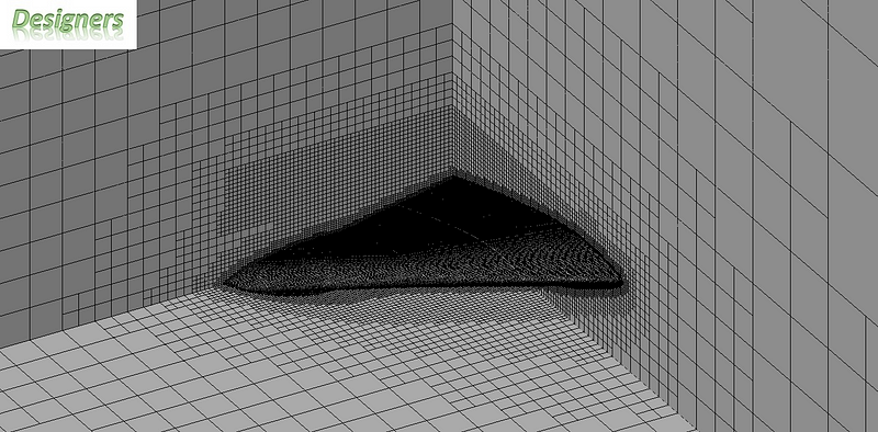
     Fig. 2 shows the computational mesh along with the computational domain. The surface mesh is also shown with Fig. 2. It can be seen that the mesh is refined in the areas of interests and in the wake of the aircraft to properly capture the relevant flow features. The Cartesian mesh with immersed boundary method, cut-cell approach and octree refinement is used for creating the mesh. The mesh has 6.5 million cells, of which around 0.71 millions cells are at boundary of the aircraft.

     The simulations employ κ-ε turbulence model with damping functions and two-scales wall functions. SIMPLE-R (modified) as the numerical algorithm. Second order upwind and central approximations as the spatial discretization schemes for the convective fluxes and diffusive terms. The software solves the Favre-averaged Navier-Stokes equations to predict turbulent flow. The simulations are performed to predict three-dimensional steady-state flow over the aircraft

Fig. 2, Dashed lines indicate symmetry boundary conditions

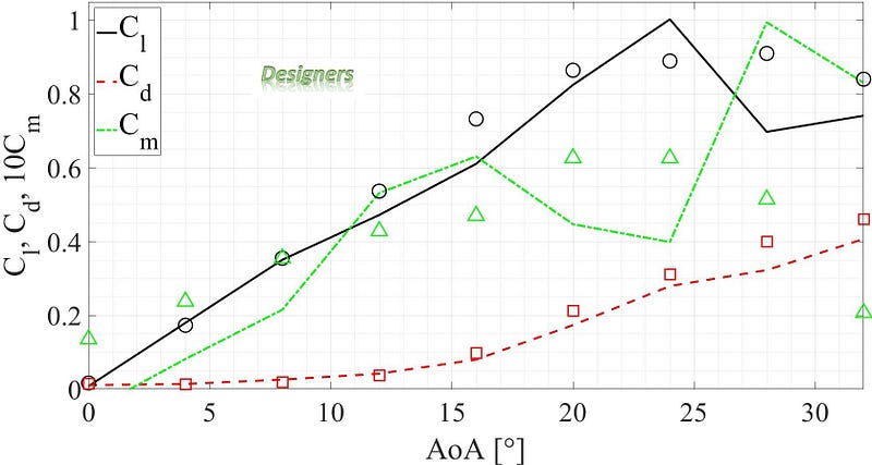
     Angle of attack of 7 and 17 degrees are considered. At 7 degree angle of attack, the drag life and moment coefficients are within 6, 8 and 12% of the published data, respectively. For 17 degree angle of attack, the coefficients are within 4, 7, 33% of the published data [3, 4]. On average, the results of the present simulations are within 6% of the published data for force coefficients and within 12% in terms of pitching moment coefficient. The pitching moment coefficient will improve with refinement of the mesh, as shown by [3]; which I will do if ever I convert this into a manuscript 😂. The post processing from CFD simulations is shown in Fig. 3-4. Within Fig. 3, the iso-surfaces represent vorticity in the direction of flow, colored by pressure. The direction of flow is shown by black arrows. Streamlines colored by vorticity are also visible. It can be seen from Fig. 2 that the simulation captures important flow features such as vortex formation very accurately, in such small number of mesh cells. Fig. 4 shows wing of the velocity iso-surfaces colored by vorticity in the direction of flow, focused around the wing.

Fig. 3, Alternating 7 and 17 degree angles of attacks

Fig. 4, Top-Bottom, 17 and 7 degrees angle of attack

     The simulations are solved using 10 of 12 threads of a 4.0 GHz CPU with 32 GB of total system memory of which almost 30 GB remains in use while the simulations are in progress. To solve each angle of attack, 3 hours and 47 minutes are required.

Update 01

     Formation flight simulation is performed with 7.3 million cells (limited by RAM). Symmetry boundary condition is used to simulate only the area of interest. The mesh and computational domain is shown in Fig. 5. Within Fig. 5, dashed lines indicate symmetry boundary condition.

Fig. 5, Airliners in formation flight mesh and computational domain

     The results show that the leading aircraft has 16.52% more drag than the trailing aircraft. The results also show that the the leading aircraft has 5.4% less lift than the trailing aircraft. However, the leading aircraft produces 2.4% more lift than the airliner flying without the trailing aircraft (flying solo). The leading aircraft also produces 3% less drag than the airliner flying solo. These results are at 7 degree angle of attack. Whether these results are fruitful aero-structurally, remains to be seen. The post processing from simulations are shown in Fig, 6.

Fig. 6, Top-Bottom, 17 and 7 degrees angle of attack

     Within Fig. 7, surface plots represent pressure, velocity streamlines indicate vortices, iso-surfaces show vorticity magnitude in the direction of flight.

     Thank you for reading, If you would like to collaborate on projects, please reach out.

References

[1] Doug Lacy and Adam M. Clark, "Definition of Initial Landing and Takeoff Reference Configurations for the High Lift Common Research Model (CRM-HL)", AIAA Aviation Forum, AIAA 2020-2771, 2020 10.2514/6.2020-2771

[2] 4th AIAA CFD High Lift Prediction Workshop Official Test Cases, https://hiliftpw.larc.nasa.gov/Workshop4/OfficialTestCases-HiLiftPW-4-2021_v15.pdf

[3] K. Goc, S., T. Bose and P. Moin, "Large-eddy simulation of the NASA high-lift common research model", Center for Turbulence Research, Stanford University, Annual Research Briefs 2021

[4] 4TH High Lift Workshop Results, ADS, https://new.aerodynamic-solutions.com/news/18