Computational Fluid Dynamics (CFD) Analysis of a Horizontal Axis Tidal Turbine (Update 01)

     In this post, the results of numerical simulations carried out on a three-blade horizontal-axis tidal turbine blades are made available. These simulations are a part of larger project relating to a horizontal-axis tidal turbine.

 

     The turbine under investigation had a diameter of 4 m. The aero-foils employed include the NACA 4424 (chord length 0.25 m), NACA 4420 (chord length 0.2312 m), NACA 4418 (chord length 0.2126 m), NACA 4417 (chord length 0.1938 m), NACA 4416 (chord length 0.175 m), NACA 4415 (chord length 0.1562 m), NACA 4414 (chord length 0.1376 m), NACA 4413 (chord length 0.1188 m) and the NACA 4412 (chord length 0.1 m) at a distance of 0.4 m, 0.6 m, 0.8 m, 1 m, 1.2 m, 1.4 m, 1.6 m, 1.8 m, 2 m from the blade root, respectively [1].

 

     The numerical simulations were carried out on SolidWorks Flow Simulation Premium software. The software employs κ-ε turbulence model with damping functions, SIMPLE-R (modified) as the numerical algorithm and second order upwind and central approximations as the spatial discretization schemes for the convective fluxes and diffusive terms. The time derivatives are approximated with an implicit first-order Euler scheme. To predict turbulent flows, the Favre-averaged Navier-Stokes equations are used. The software employs a Cartesian mesh which is created using the immersed boundary method.

 

     The simulations were carried out using the Local rotating region(s) (Sliding) technique. The mesh had a total of 589,763 cells. 132,045 cells were at the turbine blade-rotating region boundary. While the process of mesh generation, a mesh control was employed to refine the mesh near the turbine blades and at the boundary of the rotating region and the stationery computational domain. To refine the mesh for the mesh independent test, the curvature level was increased i.e. the mesh in the areas of interest was refined by a factor of 8. As a result, the refined mesh had a total of 916,577 cells. A total of 221,978 were present around the turbine blade. The computational mesh around the turbine blade is shown in Fig. 1. The refined mesh in the areas of high gradients is also clearly visible. The computational domain had dimensions of 2D x 2D x 2.4D, where D is the diameter of the turbine. The dimensions for the computational domain resemble to those in [2].

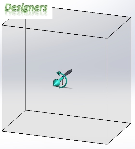
     Fig. 2 shows computational domain around the turbine blades. In Fig. 2, the curved teal arrow represents the direction of rotation of the turbine. The green arrows represent the respective co-ordinate directions. The brown arrow represents the direction of the force of gravity. The blue arrow represents the direction of the fluid velocity. The circular disc represents the rotating region.

 

Fig. 1, The computational mesh.

    

Fig. 2, The computational domain and the orientation of the boundary conditions.

 

     The simulations were carried out for a total of 5 tip-speed ratios for the turbine ranging from 2 to 10. The fluid; water, velocity was set at 2 m/s. The results are indeed, mesh independent. The mesh independence test was conducted on the design point of the turbine i.e. at the TSR of 6. The plot between the turbine tip-speed ratio; TSR, and the co-efficient of power is shown in Fig. 3. It can be clearly seen from Fig. 3 that the results are in close agreement with the results from [1, 3]. The CFD results from both studies are lower then the BEM, Blade-Element Momentum, results because the three-dimensional effects are not considered while implementing the BEM method.

 

Fig. 3, Turbine efficiency plot.

 

     Fig. 4 shows velocity streamlines colored by velocity magnitude, both of these features are drawn relative to the rotating reference frame, around the turbine blade cross-section at various tip-speed ratios. It can be seen from Fig. 4 that the turbine stalls at TSR of 2 due to a large positive angle of attack. It can also be seen that as the TSR increases, the angle of attack on the blade decreases, it is because of this reason that the power output from the turbine increases.

 

 

Fig. 4, Row 1, L-R; TSR of 2 and 4. Row 2, L-R; TSR of 6 and 8. Row 3, TSR of 10.

 

     Thank you for reading. If you would like to collaborate with research projects, please reach out.

     [1] Binoe E. Abuan, and Robert J. Howell, "The Influence of Unsteady Flow to the Performance of a Horizontal Axis Tidal Turbine," Proceedings of the World Congress on Engineering. London, 2018.

     [2] Ibrahim, I. H., and T. H. New, "A numerical study on the effects of leading-edge modifications upon propeller flow characteristics," Proceedings of Ninth International Symposium on Turbulence and Shear Flow Phenomena. Melbourne, 2015.
     [3] Bahaj, A., Batten, W., & McCann, J. (2007). Experimental verifications of numerical predictions for the hydrodynamic performance of horizontal axis marine current turbines. Renewable Energy, 2479-2490.

Update 01:

     CFD post processing added. One more TSR simulated.

Steady-State VS Transient Propeller Numerical Simulation Comparison

     This post is about the comparison between steady-state and transient computational fluid dynamics analysis of two different propellers. The propellers under investigation are 11x7 and 11x4.7 propellers. The first number in the propeller nomenclature is the propeller diameter and the second number represents the propeller pitch, both parameters are in inch. The transient analysis was carried out using the sliding mesh technique while the steady-state results were obtained by the local rotating region-averaging method. For details about 11x7 propeller click here, for the details about 11x4.7 propeller, click here.

 

     As expected, the propeller efficiencies of transient and steady-state analysis are within 0.9% of each other, as shown in Fig. 1-2. Therefore, it is advised to simulate propellers and horizontal axis wind turbines using the steady-state technique as long as no time-dependent boundary conditions are employed.

 

Fig. 1, Propeller efficiency plot.

  

 Fig. 2, Propeller efficiency plot.

 

     It can be seen from Fig. 3-4 that time taken by the steady-state simulation to converge is on average 42.37% less that the transient analysis.  The steady-state analysis takes considerably less time to give a solution then a transient analysis.

 

Fig. 3, Solution time.

 

Fig. 4, Solution time.

 

Thank you for reading. If you would like to collaborate on research projects, please reach out.

SolidWorks Flow Simulation Premium: Propeller/Horizontal Axis Wind Turbine CFD Tutorial

The tutorial is in the attached video. Analysis such as: 11x7 Aeronautic Propeller Characteristics, 11x4.7 Aeronautic Propeller Characteristics and Wind Turbine SolidWorks Flow Simulation Premium Computational Fluid Dynamics are setup using the same method.

11x7 Aeronautic Propeller Characteristics (Using CFD) (Verified and Validated) (Update 02)

     This post presents the results from an aeronautic propeller CFD analysis.

    
     An 11x7 propeller was modelled using SolidWorks CAD package using the geometry from [1]. The simulations were run at two different rotational velocities and each rotational velocity was simulated at three advance ratios. The mesh for the 3,000 RPM rotational velocity had 213,205 total cells among which 24,048 cells were at the solid fluid boundary. While, the mesh for the 5,000 RPM rotational velocity had 369,963 total cells among which 68,594 cells were at the solid fluid boundary. A mesh control was employed to refine the mesh near the propeller geometry and at the boundary of the rotating region and the stationery domain for all of the cases simulated. This was done to ensure accuracy of the results was within an acceptable range. The results of the numerical simulations are plotted along with the experimental results [1] in Fig. 1.

Fig. 1 J= Advance Ratio, η_prop = propeller efficiency

     It can be seen from Fig. 1 that the trends for the propeller efficiency are in agreement with the experimental results. To increase the mesh density for the mesh independence test, the number of cells in  each of the respective co-ordinate directions was increased by a factor of 1.1. The mesh is shown in the Fig. 2.

Fig. 2 The computational mesh around the propeller.

     The computational domain size was at 2D x 2D x 2.4D, D being the propeller diameter, as shown in Fig. 3. In Fig. 3, the curved teal arrow represents the direction of rotation of the sliding mesh. The blue arrow represents the direction of free stream velocity while the brown arrow represents the force of gravity.

 Fig. 3 The computational domain.

Fig. 4 The pressure distribution and the velocity vectors around the propeller.

     The CAD model files and the simulation setup files for the numerical analysis are available here.

     Thank you for reading. If you'd like to collaborate on research projects, please reach out.

[1] Brandt, J. B., & Selig, M. S., “Propeller Performance Data at Low Reynolds Numbers,” 49th AIAA Aerospace Sciences Meeting, AIAA Paper 2011-1255, Orlando, FL, 2011.

doi.org/10.2514/6.2011-1255

 

Update 01

     Results from the mesh independent study are now available.

Update 02

     CAD model files are now uploaded. The CFD simulation setup files are also included.