The Aerofoil

     Aerofoil, a simple geometric shape that is responsible for heavier than air flight and energy generation from of wind, hydraulic and steam turbines. However, much mystery and confusion exists about how the aerofoil works. Here an explanation is presented about the working of an aerofoil by using computational fluid dynamics and without using any equations.

     The fluid bends and tends to follow the shape of an object placed in its path when the fluid flows around the said object such as an aerofoil. This phenomenon happens due to the Coanda effect. Fig. 1 shows streamlines around an aerofoil at a Mach number of 0.22 and Reynolds number of 5e6. It can be seen from Fig.1 that the fluid starts to bend as soon as it reaches the leading edge of the aerofoil and the fluid follows the shape of the aerofoil.

Fig. 1, The white arrows represent the direction of fluid flow.

     It is well understood that, as a moving fluid bends (changes direction), a pressure difference is created across the flow path. To understand this better, consider a tornado or a typhoon (not the aircrafts). In a tornado, the fluid revolves around a central axis. Consider a point at the center of the tornado. As this point moves towards the circumference of the tornado i.e. away from the center, the pressure increases and vice-versa. This happens due to the curvature of the streamlines inside a tornado. The more the curvature difference, the more the pressure difference across the streamlines.

     In the case of symmetric aerofoils (which have top and bottom half at the same shape), there is no lift generated because the curvature of the streamlines is same on both the suction (top) and pressure (bottom) sides of the aerofoil. The resulting pressure difference between the suction and the pressure sides is zero. This can be seen in the negative coefficient of pressure (-C_p) plot shown in Fig. 2. The coefficient of pressures can be seen to overlap. This plot and subsequent figures and plots are generated using the data obtained from the computational fluid dynamics analysis of the aerofoil. Fig. 3 shows pressure distribution around the aerofoil. It is quite clear that the pressures at the top and bottom surface of the aerofoil are same, hence no lift generation. It is also evident that a pressure difference exists between leading and trailing edge of the aerofoil, hence the presence of the drag force (pressure drag) even at no angle of attack.

Fig. 2, Along the horizontal axis, 0 refers to leading edge.

Fig. 3, Air flow is from left to right.

     But, if the same aerofoil is placed at an angle to the flow, the curvature of the streamlines change, as visible in Fig. 4. Due to the different curvature on the suction and pressure side of the aerofoil, a pressure gradient in created between the suction and pressure side of the aerofoil with lower pressure at the top and higher pressure at the bottom, as shown in Figs. 5. The -C_p plots for the aerofoil at the angle of attack is shown in Fig. 5. The pressure difference is quite clear in both Figs. 5-6.

Fig. 4, The white arrows represent direction of fluid flow.

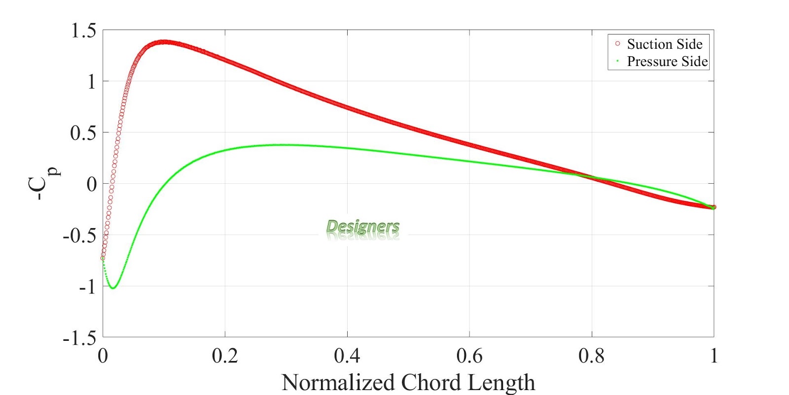
Fig. 5, Along the horizontal axis, 0 refers to leading edge.

Fig. 6, Air flow is from left to right.

     In the far field, the pressure is uniform, colored by green in Figs. 3, 6. In a case when the fluid is turning, the pressure increases as away from the center of the curvature and vice versa. Looking at the suction side, the pressure will decrease as distance to the center increases. The pressure gradient at the bottom can be explained by the same reason. This difference in pressure is what causes the lift force, as evident from Fig. 5.

     Velocity distribution around the aerofoil at an angle of attack is shown in Fig. 7. It can be seen that the fluid has more velocity at the suction side of the aerofoil as compared to the pressure side. The velocity distribution on the aerofoil without an angle of attack is same on both the pressure and suction sides of the aerofoil and is shown in Fig. 8.

Fig. 7, Air flow is from left to right.

Fig. 8, Air flow is from left to right.

     

     This again, can be explained by the pressure gradient. It can be seen from Figs. 5-6 that the pressure gradient at the suction side of the aerofoil is much more favorable as compared to the pressure side. It can be seen from Figs. 5-6 that the pressure is highest at the leading edge of the aerofoil (stagnation point). The pressure falls to its lowest magnitude past the leading edge of the aerofoil on the suction side. Meanwhile, on the pressure side, the pressure drop is less severe as compared to the suction side. As a result, the fluid faces less resistance on suction side of the aerofoil in comparison with the pressure side. This is the reason why fluid velocity is more at the top as compared to the bottom of the aerofoil, not vice versa. In all the figures, the color red means maximum magnitude and the color blue implies minimum magnitude.

If you want to collaborate on the research projects related to turbomachinery, aerodynamics, renewable energy, please reach out. Thank you very much for reading.

Aerofoil Kinematics Computational Fluid Dynamics (Update: 01)

This post is about a 2D NACA 0010 aerofoil undergoing various forms of forced kinematics i.e. pure heaving and pitching and a combination of two known as flapping.

Heaving motion is achieved by changing the angle of attack on the aerofoil based on the Eqn. 1.

α_e = arctan[2*π*St_a*cos(2*π*f_h*t)] + α_i               Eqn. 1

The pitching motion is achieved by employing the sliding mesh with the rotational velocity governed by Eqn. 2.

ω = 2*π*f_h*ϑ*cos(2*π*f_h*t)                                 Eqn. 2

w.r.t. Eqn. 1-2 α_e is the effective angle of attack, St_a is Strouhal number (defined as (f_h*h0/U∞)), f_h is the frequency of oscillations, while ω, t and ϑ represent rotational velocity, instantaneous time and pitching angle. h0 is the heaving amplitude and U∞ is the free stream velocity.

The flapping motion is achieved by a combination of the heaving and pitching. In this particular simulation, the aerofoil is in the power extraction mode, meaning the feathering parameter χ is greater in magnitude than 1.0. Feathering parameter is defined by Eqn. 3.

χ = ϑ/arctan(h0*2*π*f_h/U∞)                                  Eqn. 3

The boundary conditions employed for the set of simulations are at Re 50,000, St_a 0.0149, h0 = aerofoil chord length, χ = 1.1 and f_h = 0.5 Hz. The animation of the velocity contours superimposed with streamlines is shown in Fig. 1. The velocity scale ranges from 0 to 7 m/s. Pressure distribution around the aerofoils in various forms of motion, after five complete cycles is shown in Fig. 2.

Fig. 1, Flow animation, fluid flow direction is from left to right

Fig. 2, Fluid flow is from left to right

If you want to collaborate on the research projects related to turbomachinery, aerodynamics, renewable energy, please reach out. Thank you very much for reading.

Heaving Airfoil Simulation

This post is about a 2D NACA 0012 heaving aerofoil. Heaving motion is achieved by changing the angle of attack on the aerofoil based on the Eqn. 1.

α_e = arctan[2*π*St_a*cos(2*π*f_h*t)]+ α_i               Eqn. 1

w.r.t. Eqn. 1, α_e is the effective angle of attack, St_a is Strouhal number, f_h is the heaving frequency.

The case S1 and H6 from [1] are compared in the animations below.

If you want to collaborate on the research projects related to turbomachinery, aerodynamics, renewable energy, please reach out. Thank you very much for reading.

References

[1] https://doi.org/10.1121/10.0001419

Formation Flight Computational Fluid Dynamics

     This is a post about computational fluid dynamics analysis of formation flight.

     The results from an analysis of three unmanned combat aerial vehicles (UCAVs) flying in a V-type formation are presented. The chosen UCAV configuration, shown in Figs. 1-2 and available for download here, is named SACCON (Stability And Control Configuration) UCAV. This configuration is used because of the availability of the geometric and aerodynamic data, used in the validation and verification of the numerical analysis. The SACCON UCAV is designed by NATO's (North Atlantic Treaty Organization) RTO (Research and Technology Group) under Applied Vehicle Task Group (AVT-161) to assess the performance of military aircrafts.

Fig. 1, SACCON UCAV

Fig. 2, Technical drawing for the SACCON UCAV

     The simulation is performed using commercially available computational fluid dynamics code.  The details about the solver and the discretization schemes are presented next. The simulation is performed using SIMPLE-R solver for pressure-velocity coupling. The diffusive terms of the Navier-Stokes equations are discretized using central differentiating scheme while the convective terms are discretized using the upwind scheme of second order. The κ-ε turbulence model with damping functions is implemented to model turbulence. The simulation predicts three-dimensional steady–state flow over UCAVs.

     The Reynolds and Mach number of flow are set at 1e6 and 0.15, respectively. The two trailing UCAVs are placed 3 wingspans behind the leading UCAV. The trailing UCAVs are a wingspan apart. The V-type configuration is chosen because it is the most common observation in birds (author's observation). The V-type formation is shown in Fig. 3. All three UCAVs are at 5° angle-of-attack.

Fig. 3, The V-type formation (top view)

     The boundaries of the computational domain are located at a distance equivalent to 10 times the distance between the nose of the leading UCAV and the tail of the trailing UCAV. The mesh is made of 821,315 cells. Mesh controls are used to refine the mesh in the areas of interest i.e. on the surfaces of the UCAVs and in the wake of all three UCAVs. A cartesian mesh with immersed boundary method is used for the present study. The computational domain with mesh is shown in Fig. 4 while a closeup of the mesh is shown in Fig. 5.

Fig. 4, The computational domain and mesh

Fig. 5, Closeup of mesh, notice the refined wakes of the UCAVs

     For validation and verification, the lift and drag forces from the present study are compared with studies [1-2]. The results are in close agreement with [1,2] As a result of flying in a formation, an improvement in the lift-to-drag ratio of 10.05% is noted. The lift-to-drag ratio of the trailing UCAVs is at 11.825 in comparison with a lift-to-drag ratio of a single UCAV, i.e. 10.745. The lift coefficient is increased by 7.43% while the drag coefficient decreased by 2.174%. The reason(s) to why the efficiency increases will be looked upon later, if ever the author has the time and will power ☺.

     The results from post processing of the simulations are presented in Figs. 6-7. The pressure iso-surfaces colored by velocity magnitude are shown in Fig. 6. While the velocity iso-surfaces colored by pressure magnitude are shown in Fig. 7.

Fig. 6, Flight direction towards the reader

Fig. 7, Flight direction away from the reader

     Thank you very much for reading. If you would like to collaborate on research projects, please reach out.

[1] https://doi.org/10.2514/1.C031386

[2] https://doi.org/10.1155/2017/4217217