Showing posts with label immersed boundary method. Show all posts

Monday, 7 July 2025

A Simplified Immersed Boundary Method using Ray Casting

     Yours truly is an avid gamer, @fadoobaba (YouTube). The ray casting algorithm๐Ÿ›ธ; a fundamental ๐Ÿงฑ technique used in video game ๐ŸŽฎ development and computer graphics, has been implemented within the finite difference method ๐Ÿ code yours truly has been developing. In abundant spare time, of course๐Ÿ˜ผ. In this post, this method is explained. For details about ray casting using matplotlib.path, refer to here. For validation of the code, refer to here, backwards-facing step, curved boundaries, here (moving cylinder) and here.

NOTE: This method requires a GPU, if dear readers don't have a GPU then please stop being peasants... ๐Ÿ™‰

     If you plan to use these codes in your scholarly work, do cite this blog as:

     Fahad Butt (2025). S-IBM (https://fluiddynamicscomputer.blogspot.com/2025/07/a-simplified-immersed-boundary-method.html), Blogger. Retrieved Month Date, Year

     The first step is to setup the polygon ๐Ÿ . The polygon = cp.column_stack((x1, y1)) statement is used to combine x1 and y1 into a single array representing the polygon vertices. The following statements are used to store the x and y coordinates of the polygon vertices and nvert is the total number of vertices.

px = polygon[:, 0]

py = polygon[:, 1]

nvert = len(polygon)

     The boolean masks ๐Ÿ‘บ are then initialized. The following arrays track whether a grid point is inside the polygon based on horizontal and vertical ray intersections. False = outside ❌, True = inside ✅. Then a loop is implemented to for each edge ๐Ÿ“ of the polygon, defined by vertices i (current) and j (previous), with % nvert ensuring the polygon is closed (last vertex connects back to the first). (xi, yi) and (xj, yj) define the current edge and previous edge.

horizontal_inside = cp.zeros_like(test_x, dtype=bool) 

vertical_inside = cp.zeros_like(test_x, dtype=bool) 

for i in range(nvert):

    j = (i - 1) % nvert

xi, yi = px[i], py[i]

xj, yj = px[j], py[j]

     A check ⁉️ is performed to ensure a ray crosses the polygon edge once. cond1 statement checks if the test point lies between the y-values of the edge's endpoints i.e., a ray could cross it. intersect_x finds where the edge crosses a horizontal line at test_y. cond2 checks if the intersection lies to the right of the test point. ^= is XOR toggles the "inside" state each time the ray crosses an edge. The addition of small term ~1e-16 prevents division by zero for horizontal edges. Similar method is applied to verify the points using vertical ray. cond3 checks if the edge crosses a vertical ray (top to bottom) from (test_x, test_y). slope1 and intersect_y computes where the vertical ray at x=test_x intersects the edge. A point is inside only if both horizontal and vertical rays classify it as inside. A point is considered inside the foil only if both ray checks are true. curve is the 2D boolean mask of grid points inside the foil body.

cond1 = ((yi > test_y) != (yj > test_y))

slope = (xj - xi) / (yj - yi + 1e-16)

intersect_x = slope * (test_y - yi) + xi

cond2 = test_x < intersect_x 

horizontal_inside ^= cond1 & cond2

cond3 = ((xi > test_x) != (xj > test_x))

slope1 = (yj - yi) / (xj - xi + 1e-16)

intersect_y = slope1 * (test_x - xi) + yi

cond4 = test_y < intersect_y

vertical_inside ^= cond3 & cond4

inside = horizontal_inside & vertical_inside

curve = inside.reshape(X.T.shape)

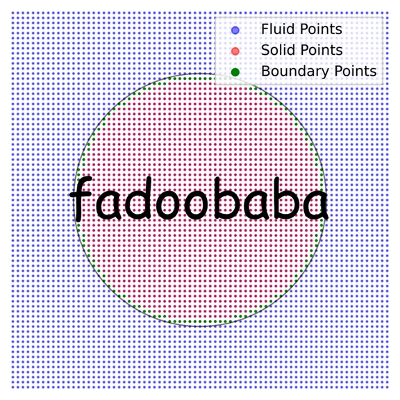
     Using both horizontal and vertical rays reduces false positives (e.g., near sharp corners). The & ensures only points unambiguously inside are marked. Within Fig. 1, the points on the shape boundary, points inside ๐Ÿชฐ and outside ๐ŸŒ the shape boundary are shown. A point is a boundary if it is inside the body, but any of its neighbors is outside. Following statements are used to mark the boundary of the object. Boundary detects the "skin" of the body for applying no-slip, force, or stress conditions.

interior = curve[1:-1, 1:-1]

right = curve[2:, 1:-1]

left = curve[:-2, 1:-1]

top = curve[1:-1, 2:]

bottom = curve[1:-1, :-2]

boundary = interior & ~(right & left & top & bottom)

     The statements boundary_indices = cp.where(boundary_mask) ... valid_right = (boundary_indices[0] + 1 < X.shape[0]) & (~curve[right_neighbors]) ... etc. extract boundary indices and their valid neighbors i.e. these lines extract the (i, j) grid indices of the surface and locate which neighbor cells are valid fluid neighbors (outside the body and within domain bounds). These are needed to compute normals or apply boundary conditions via interpolation or extrapolation from the fluid.
Fig. 1, Mesh cells


     For validation of the results from present simulations, the case of flow around a circular cylinder is selected. Fig. 1 shows the results from the code at Re 200. The drag coefficient obtained from this code is 1.396 while from the literature, the value is at 1.4 [1]. The lift coefficient from the code is at 0.000134. Within Fig. 2, top row shows u and v velocity components and bottom row shows pressure and vorticity.


Fig. 2, The flow-field

     For the second an more complex validation case, a swimming fish is simulated. The lift and drag coefficients obtained from the simulation are compared with experimental results. The drag coefficient from the current code is at 0.342 while from the published literature, the value is at 0.348. Maximum lift coefficient is at 7.243 and 8 from the present code as compared to the published literature [2]. Within Fig. 3 the u and v velocities, pressure and velocity streamlines are shown for St = 0.8 and Reynolds number of 500. The computational mesh near the fish is shown in Fig. 4. Within Fig.4, a zoomed in view towards the right shows the mesh at the trailing edge of the fish.
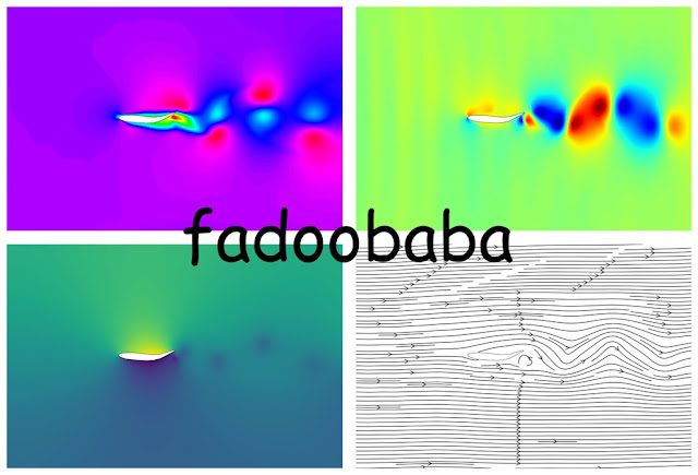

Fig.3, Post-processing of results

Fig. 4, The mesh

     This method allows handling arbitrary deforming / non-deforming shapes on a fixed Cartesian grid. In summary, the method has the following steps.

1. Generate polygon shape (e.g., airfoil, cylinder)

2. Flatten mesh for vectorized testing

3. Use ray casting to check if points are inside shape

4. Build a boolean mask of body region

5. Identify surface (boundary) points

6. Extract boundary indices for physics coupling


References

     [1] Braza M, Chassaing P, Minh HH. Numerical study and physical analysis of the pressure and velocity fields in the near wake of a circular cylinder. Journal of Fluid Mechanics. 1986;165:79-130. doi:10.1017/S0022112086003014

     [2] Fulong ShiJianjian XinChuanzhong OuZhiwei LiXing ChangLing Wan; Effects of the Reynolds number and attack angle on wake dynamics of fish swimming in oblique flows. Physics of Fluids 1 February 2025; 37 (2): 025205 doi.org/10.1063/5.0252506

     Thank you for reading! If you want to hire me as a post-doc researcher in the fields of thermo-fluids and / or fracture mechanics, do reach out!

Monday, 26 May 2025

A Simplified Immersed Boundary Method (S-IBM)

     In this post, details will be shared about a simplified version of the Immersed ๐Ÿคฟ Boundary Method for fluid dynamics ๐Ÿ’จ simulations which yours truly has developed in abundant spare time ⏲, referred to as S-IBM ๐Ÿค“. The purpose of this code is for teaching ๐ŸŽ“ purposes only. The mesh is Cartesian and the method used has no measures in place to resolve the stairstep ๐“Š mesh. The syntax share in this post is for Python ๐Ÿ, but this code can be translated to other languages such as C or MATLAB, easily.

     The process starts with creating a polygon, a circular cylinder ⭕ for this post. A polygon is created using parametric equations for the circle. NOTE: Before writing these lines, several parameters such as domain size, mesh size, number of points in each coordinate direction etc. have been already defined and calculated. For more information, read here.

theta = np.linspace(0, 2 * np.pi, 100) # create equally spaced angles from 0 to 2 * pi

radius = 0.5; # radius of circle

circle_center_x = 3.3 # circle center x

circle_center_y = D / 2 # circle center x

x1 = circle_center_x + (radius * np.sin(theta)) # x-coordinates

y1 = circle_center_y + (radius * np.cos(theta)) # y-coordinates

     Path from matplotlib is used to create a polygon approximation of a circle or an airfoil by using the x and y co-ordinates of the circle (x1, y1) or any shape. Next, coordinate pairs of the grid points are created using vstack and ravel commands. A check is performed to verify if a grid point falls inside the polygon. custom_curve is a boolean array. The values inside this array are True only for the points inside the polygon. Transpose is used to keep the curve orientation consistent with the Navier-Stokes equations.

circle_path = Path(np.column_stack((x1, y1)))

points = np.vstack((X.ravel(), Y.ravel())).T

custom_curve = circle_path.contains_points(points).reshape(X.shape)

curve = custom_curve.T

     Another boolean mask is created for boundary points using the boundary_mask statement. Points that are inside the polygon (circle) are marked using using the interior statement.

boundary_mask = np.zeros_like(curve, dtype=bool)

interior = curve[1:-1, 1:-1]

     Next a check is performed to mark each interior point's immediate neighbor. right means point to the right of each interior point, bottom means point to the bottom of each interior point etc. boundary statement is used to identify the boundary points (fluid-solid interface) according to the following logic. The point itself is inside the circle (interior = True) and at least one neighbor is outside. boundary_mask[1:-1, 1:-1] is used to fill the boolean with boundary. Consider a 5×5 a grid (zoomed near the polygon boundary). X marks solid points (inside circle), O marks fluid points, as shown in Fig. 1. For example, if interior = True, right = True, left = True, top = True and bottom = True → boundary = True & ~(True) = False i.e. an interior point. And for example, interior = True, right = False, left = True, top = True, bottom = True → boundary = True & ~(False) = True, i.e. a point on the right boundary. For points outside the polygon, interior = False → boundary = False (regardless of neighbors).


Fig. 1, A grid example

right = curve[2:, 1:-1]

left = curve[:-2, 1:-1]

top = curve[1:-1, 2:]

bottom = curve[1:-1, :-2]

boundary = interior & ~(right & left & top & bottom)

boundary_mask[1:-1, 1:-1] = boundary

custom_curve_boundary = boundary_mask

     In the next step, boundary_indices obtains indices of all boundary points. right_neighbors, left_neighbors etc. calculates indices of neighboring points in all directions. valid_right, valid_left etc. checks if the neighbor is within domain bounds (not at edge) and is outside the circle (fluid point). This allows proper application of no-slip boundary conditions. If for example, valid_right is True, pressure is taken from the right neighbor to be applied to the corresponding boundary index. A visualization of the points is shown in Fig. 2.

boundary_indices = np.where(custom_curve_boundary)

right_neighbors = (boundary_indices[0] + 1, boundary_indices[1])

left_neighbors = (boundary_indices[0] - 1, boundary_indices[1])

top_neighbors = (boundary_indices[0], boundary_indices[1] + 1)

bottom_neighbors = (boundary_indices[0], boundary_indices[1] - 1)

valid_right = (boundary_indices[0] + 1 < X.shape[0]) & (~curve[right_neighbors])

valid_left = (boundary_indices[0] - 1 >= 0) & (~curve[left_neighbors])

valid_top = (boundary_indices[1] + 1 < X.shape[1]) & (~curve[top_neighbors])

valid_bottom = (boundary_indices[1] - 1 >= 0) & (~curve[bottom_neighbors])


Fig. 2, Depiction of grid points in various regimes


     While plotting Fig. 2, several points are skipped. This is done to make plot clearer. This code can be easily implemented in other languages such as MATLAB (inpolygon), C (ray-casting) etc. At Re 200, this code predicts a Drag coefficient of 1.395 and a Lift coefficient of 0.053. These values are well within rage of the values reported by [1]. In this code, there is no interpolation of scheme or smoothing employed. The lift and drag force coefficients for one shedding cycle are shown in Fig. 3. Within Fig. 4, u and v velocities (top left and right), pressure and streamlines (bottom left and right) are shown. 


Fig. 3, red = Cd and black = Cl

Fig. 4, Post processing from the simulations.

References

[1] Braza M, Chassaing P, Minh HH. Numerical study and physical analysis of the pressure and velocity fields in the near wake of a circular cylinder. Journal of Fluid Mechanics. 1986;165:79-130. doi:10.1017/S0022112086003014

     Thank you for reading! If you want to hire me as a post-doc researcher in the fields of thermo-fluids and / or fracture mechanics, do reach out!