Monday 26 March 2018

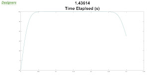
1D Transient Diffusion (MATLAB code)


clear; clc;% clear the screen and memory

Nx=500; %number of space nodes

Nt=10000; %number of time nodes

Lx=0.3; %length of space (m)

Lt=10; %length of physical time (s)

dx=Lx/(Nx-1); %grid spacing

dt=Lt/(Nt-1); %time step

c=0.000097; %speed of wave (constant)

a=c*dt/dx.^2;

u=100*ones(Nx,1); %initialization of matrix for the property under investigation

x=zeros(Nx,1); %initialization of space

for i=1:Nx-1 %space loop

    x(i+1)=x(i)+dx;

end

u(1)=-20; %boundary condition

u(Nx)=50; %boundary condition

for t=0:dt:Lt %time loop

    un=u; %u(i,t)

    for i=2:Nx-1 %solution loop, backward in space forward in time

        u(i)=((1-2*a)*un(i))+a*(un(i+1)+un(i-1)); %discretized equation, u(i,t+1)

    end

    plot(x,u) %plotting

    title({t;'Time Elaplsed (s)'},'FontSize',38.5);

    pause(0.001)

end


Friday 23 March 2018

1D non-Linear Convection (MATLAB code)


clear; clc;% clear the screen and memory

Nx=41; %number of space nodes

Nt=82; %number of time nodes

Lx=2; %length of space (m)

Lt=1; %length of time (s)

dx=Lx/(Nx-1); %grid spacing

dt=Lt/(Nt-1); %time step

a=dt/dx;

u=ones(Nx,1); %initialization of solution matrix

x=zeros(Nx,1); %initialization of space

hold on

for i=1:Nx-1 %space loop

    x(i+1)=x(i)+dx;

end

for i=0.5/dx:1/dx %initial conditions

    u(i)=2;

end

for t=1:Nt %time loop

    un=u; %u(i,t)

    for i=2:Nx %solution loop, backward in space forward in time

        u(i)=un(i)-u(i)*a*(un(i)-un(i-1)); %discretized equation, u(i,t+1)

    end

    plot(x,u,'k') %plotting

    pause(0.1)

end

1D Linear Convection (MATLAB code) (Updated with CFL condition)


clear; clc;% clear the screen and memory

Nx=41; %number of space nodes

Nt=82; %number of time nodes

Lx=2; %length of space (m)

Lt=1; %length of time (s)

dx=Lx/(Nx-1); %grid spacing

dt=Lt/(Nt-1); %time step

c=2; %speed of wave (constant)

a=c*dt/dx;

u=ones(Nx,1); %initialization of solution matrix

x=zeros(Nx,1); %initialization of space

hold on

for i=1:Nx-1 %space loop

    x(i+1)=x(i)+dx;

end

for i=0.5/dx:1/dx %initial conditions

    u(i)=2;

end

for t=1:Nt %time loop

    un=u; %u(i,t)

    for i=2:Nx %solution loop, backward in space forward in time

        u(i)=un(i)-a*(un(i)-un(i-1)); %discretized equation, u(i,t+1)

    end

    plot(x,u,'k') %plotting

    pause(0.1)

end


New Code, with the CFL condition satisfied.


clear; clc;% clear the screen and memory

Nx=13; %number of space nodes

Lx=2; %length of space (m)

Lt=1; %length of time (s)

dx=Lx/(Nx-1); %grid spacing

c=2; %speed of wave (constant)

dt=dx*0.1/c; %time step, Courant number = 0.1

Nt=(Lt/dt)+1; %number of time nodes

a=c*dt/dx;

u=ones(Nx,1); %initialization of solution matrix

x=zeros(Nx,1); %initialization of space

t=zeros(fix(Nt),1); %initialization of space

hold on

for i=1:Nt-1

    t(i+1)=t(i)+dt;

end

for i=1:Nx-1 %space loop

    x(i+1)=x(i)+dx;

end

for i=0.5/dx:1/dx %initial conditions

    u(i)=2;

end

for j=0:dt:Lt %time loop

    un=u; %u(i,t)

    for i=2:Nx %solution loop, backward in space forward in time

        u(i)=un(i)-a*(un(i)-un(i-1)); %discretized equation, u(i,t+1)

    end

    plot(x,u,'k') %plotting

    pause(0.1)

end

Friday 9 March 2018

Solve PDEs using MATLAB (Code)

This is a post about a code I wrote to solve  1-D Poisson's equations. The method employed is called the finite difference method. For 1-D Laplace equation, the RHS of the equation mentioned below goes to zero. Hence all the terms in the B(i) loop equal zero. Also, B(1) and B(Nx) terms equal to the boundary conditions only. I hope this code helps you in learning something.

The example equation is mentioned below.
d2y/dx2 = x2+1 and y(0)=10, y(1)=20

The result of the code is a plot between the dependent and the independent variables, as shown in Fig. 1. The accuracy of the solutions lie around 1.5 % of the analytical solution.

%solution to 1D Poisson's equations with dirichlet boundary conditions, 2nd order accurate, uniform grid
clear; clc;
Nx=101; %Enter the number of grid points
clc;
A=zeros(Nx,Nx); %Stiffness matrix
B=zeros(Nx,1); %Dependent variable vector, also used for boundary conditions and other known terms
x=zeros(Nx,1); %Independent variable vector
x(Nx)=1; %Domain size
dx=x(Nx)/(Nx-1); %Grid spacing
B(1)=(((x(1).^2)+1)*(dx.^2))-10; %Enter the function the PDE equals to multiplied by the square of the grid spacing minus the first boundary condition
B(Nx)=(((x(Nx).^2)+1)*(dx.^2))-20; %Enter the function the PDE equals to multiplied by the square of the grid spacing minus the second boundary condition
for i=2:Nx-1 %Off boundary values for the dependent variable vector
    B(i)=((x(i).^2)+1)*(dx.^2); %Enter the function the PDE equals to multiplied by the the square of the grid spacing
end
for i=1:Nx-1 %Loop for independent variable
    x(i+1)=(i)*dx;
end
for i=1:Nx %Diagonal terms for the stiffness matrix
    A(i,i)=-2;
end
for i=1:Nx-1 %Off diagonal terms for the stiffness matrix
    A(i,i+1)=1;
    A(i+1,i)=1;
end
X=A\B;
hold on
set(gca,'FontSize',28)
xlabel('Independent Variable','FontSize',38.5)
ylabel('Dependent Variable','FontSize',38.5)
title('Dependent VS Independent Variable (d^2y/dx^2 = x^2+1)','FontSize',38.5);
plot(x,X)


Fig. 1. Plot from the code